There are multiple ways to create a list of sequential numbers in Excel. The most common one should be simply type 1 in a cell, followed by drag and drop (fill-series). Another common approach would be using a simple formula of earlier cell + 1. Although these are super easy, they have their limitations – when inserting / deleting rows in-between, the sequential numbers break… 😦
If you are using Excel 365 (or Excel 2021 or above), you should use the SEQUENCE function. This method is the best way to do so. Not only is it super easy to use, but also the sequential numbers created is (almost) unbreakable.
Let’s watch it in action in this short video:
I hope you enjoy this video. If so, please give it a thumbs up, share it, and subscribe to my channel. 😉
Only the first argument (source) is required. There are optional arguments mainly for more control of how the image will fit into the cell, which is illustrated in the next screenshot:
If you have been following my blog or YouTube channel, you may have noticed I have been inactive for almost a year… don’t worry about me. I am all good! 😊
Just that I’ve got a new role that occupies most of my time and energy. What’s the role? A picture tells a thousand words…
Haha 😂 … although the answer is only word – Father!
I will be back
No worries! I am not closing this blog. I will be back for sure! My plan is to have more short contents or videos featuring Excel365, probably on a monthly basis… Stay tuned! 🤓
A decade ago, I wrote a blog post about the same in an no-formula approach. Ten years has past and Excel has evolved so much. With Excel 365, the same task can be performed in an efficient and effective manner by using TEXTJOIN function. See screenshot below:
Did you know there are 16384 columns and 1048576 rows on a worksheet? We have the flexibility to navigate any cells within this large range! Nevertheless, this is NOT what we want some time. Think about when you have created a wonderful report or dashboard, you want your audiences to stay focus on the range with information. A simple way to achieve this is to hide all unwanted columns and rows.
Again, a picture tells a thousand words. The following GIF shows what we want to achieve:
Seriously? A simple VLOOKUP formula stated below would do. What’s the challenge?
=VLOOKUP(G3,B:E,4,FALSE)
Yes, you are right if all these tables reside on the same worksheet. What if they are sitting on different worksheets? or even on different columns?
I would say it is super challenging to create a VLOOKUP formula to lookup values from different tables in the old days. Nevertheless, with Excel 365, it’s easy!
You may download the sample workbook to follow along.
Quite a long time ago, I wrote about two different approaches of preparing dependent dropdown menu in Excel. The first approach was for non Excel365 users, while the second approach was for Excel365 users. You may refer to the post here.
In this post, I will be using the same sample workbook, solving the same problem, but by a third approach using OFFSET, an Excel function that went unnoticed. 😅
You may wonder why? Because of the limitations of the first two approaches:
For the first approach using INDIRECT function, it’s quite flexible indeed.
For example, if we have four items in the first down drop menu, then we must prepare five different tables as shown in the screenshot above. You can imagine, it may take some time to prepare the tables required when we have a super long list of items using this approach. In short, the setup process would be a major hurdle using this approach, when there is a long list of items.
For the second approach using dynamic arrays, I would say that’s very easy to setup. However, as of the date this post is written on, Data Validation does not accept input of formula using dynamic array functions such as FILTER. It means, we have to rely on helper columns (What you see in column I and beyond in the screenshot below).
This limitation makes the dependent dropdown menu NOT automatically expand with Excel Table. We need to copy down formula in column I in respond to row addition to the input table. Although not a big effort, it’s just not good enough.
By using the third approach using OFFSET function, I can bypass the hurdle of the first approach, while enjoying the simple table setup:
The challenge of this approach is probably you need to feel comfortable in writing formula like this:
And also you need to know how to convert it into a Named Range.
IMPORTANT: Pay attention to the relative cell reference H3 in the above formula . When this formula is input in the name manager dialog box, the active cell has to be in I3. This means, H3 refers to the cell that is one cell to the left of the active cell. This is critical for this to work properly.
If you want to study the details later, simply download the sample workbook, modify the contents in the table and use it.
If you want to understand how it works, its major limitation, and extra tip to make sure it works on any worksheets, please see detailed explanation below.
As an Excel blogger, I feel happy when my blog posts got shared, reposted, quoted, referenced etc in a proper manner on any platform. As most creators expect, a proper manner includes sharing via proper sharing functions, such as Share in Facebook and YouTube, Repost (formally known as Retweet) in X, or any form of explicit citations about the source. That’s a fair expectation I believe.
Nonetheless, I found two of my posts got copied and posted by the following account in X yesterday.
As you can see, that’s a word by word copy without citation of sources, nor my prior consent. Is it an act of stealing?
I replied that post once i saw it, leaving the link to my original content.
You know what afterwards? I am blocked by that account.
Don’t make me wrong, I am not interested in following that account. I just wanted to see if there are any other contents of mine being posted there as if it’s his… or as if I am posting there as part of that account.
I HAVE NO RELATIONSHIP IN ANY FORM WITH THAT ACCOUNT IN X.
My dear readers, if you happened follow that account in X, and see any of my (or any others’) contents being posted there without citation or credit given back, may I kindly ask you to leave the link of the original contents by leaving comments there. Really appreciate your time and effort!
I enjoy sharing Excel tips and tricks via blogging, videos, and posts on different social media. I am happy if you find my content useful and you share with others, but please do it in a proper way. 🙏🏻
We talked about the new function – TEXTSPLIT in the previous post. Let’s share a use case of myself in this post.
From time to time, I receive email with a long list of recipents. Occassionally, I may want to see who are in the list. The quick way is to copy the list from Outlook and paste it in Excel. When I do that, I end up with a list of Names and Email addresses in a single cell like this:
Fung Wong <FungWong@abc.com>; Ernest <ernestwong@abc.com>; bee <bee@abc.com>; Cat KY Leung <cat.ky.leung@abc.com>; Gary Sou <ahsou@abc.com>; Henry Fong <fymhenry@abc.com>; Mad Lei <mad@abc.com>; Vienna Ng <ViennaNg@abc.com>; Ben Wong <wong@abc.com>; Cat Leung <cat.leung@abc.com>; Francis Lo <francislo@abc.com>; Jacqueline Liu <jacliu@abc.com>; Jim Coral <ahjimmail@abc.com>; Jia MI <jia.mi@abc.com>; Kit Yeung <kit@abc.com>; Kwong Cora <cora@abc.com>; Lo Karen <karenlo@abc.com>
But what I want is something like this:
Before the new dynamic array functions in Excel 365, I can achieve this by a couple of techniques like Text to Columns, Copy and Paste Transpose, Flash Fill. Sound like tedious but it could be done in a minute indeed. Here’s a video I made a couple of years ago when dynamic array functions were not born.
Now, with Excel 365, you won’t believe how easy it could be to perform such task. If you accept imperfection, the solution is as simple as:
It’s a common task to split text into columns in Excel. We can do that with “Text to Columns” under Data tab. That’s very handy, however it returns only static result (good for one off task) and could not split text into rows.
With the new function “TEXTSPLIT” in Excel 365 (or latest version of Excel), we can overcome these two limitations with ease.
I will show you the common use cases for this function in the video.
I hope you like this video. If you do, please give a thumbs up, share and subscribe to my channel. 😉
If you prefer reading to wach, please continue to read. Moreover, I will walk you through with examples how to use the optional agruments for this function.
You may download a sample workbook to follow along.
One day, in a causal conversation with a colleagus, he asked me if there is any good Excel training courses recommended. Face-to-face classroom training was on top of his mind, but I asked him why not considering online training, which is more flexible and easy to follow. The next question is then, do I have any recommendation as there are so many different courses avaliable in the internet.
Indeed, there are a variety of well-structured Excel training courses available in Xelplus. Do check out Leila Gharani’s Excel courses on XelPlus. Trust me, these courses are the real deal, covering everything from the basics to complex data wizardry.
Disclosure: I make a small commission (at no additional costs to you) for students who join Leila’s course via my site, but as you know I don’t just recommend anything and everything. It has to be of outstanding quality and value, and something I can genuinely recommend. After all, if it doesn’t live up to what I’ve promised you’ll think poorly of me too and I don’t want that. Oh, and just watching the course videos won’t transform your career, you have to actually put it into practice, as if reading a cookbook won’t make you a chef.
A picture tells a thousand words. This is what we want to achieve. It is only “kind of” a paginated report because it works only on the application (Excel) but not for printing. 😅
With dynamic array and new functions in Excel 365, this task is not difficult at all. Only two functions involved. They are CHOOSEROWS and SEQUENCE functions. The spin button is not something new. It’s been in Excel for too long. Just that you may not have a chance to use it before.
Before 365, this needs to be entered into the CONCATENATE function one by one, not to mention the commas in between. With Excel 365, use the function: ARRAYTOTEXT. Bingo!
Say the range of text resides in A1:A9. All you need to input is
It is so common that we deal with crosstabs in Excel. It is good for displaying summarized data. However, if you need to further analyze the data, especially with PivotTable, you will find a crosstab not the right layout. What will you do then? Move the data one by one to the PivotTable-friendly layout?
I saw my colleague did that before. No kidding. If you are talking about just a few rows and columns, no big deal. Silly but doable. What if there are hundreds of rows and tens of columns in the crosstab? Are you going to spend the entire day just moving cells around?
Power Query comes to rescue. And unbelievably, it can be done in a minute! No kidding!
You may download a sample workbook to follow along:
Here’s the situation: We have a column of values with various lengths, from 1 to 5 letters. We want to convert that into a fixed length of, say 5 letters, padding with zero(s). The following screenshot illustrates the requirement.
How would you do it? If “IF” is on top of your mind, please continue to read as I am going to show you a few diverse ways to achieve this. The approaches I am going to show you are:
Using TEXT (works best when we have numeric values only)
Using nested IF (probably the most commonly used approach, but not necessarily the best)
Using SWITCH (an alternative to nested IF, more readable and easier to construct)
Using LET (to solve the problem step by step; and make the formula more readable)
Using basic functions and logic (this is what I recommend)
The importance of explicit data type in Power Query
What could go wrong when we have a column of “ANY” data type in Power Query? Well, it depends. Depends on what? Sometimes luck! 😅
What’s wrong here?
This query has been working well all the time until one day…
A real story of myself
One day a colleague called me for the following error message that stopped the queries from running in her Power BI report.
I helped her build that Power BI report quite some time ago. She has been updating the data sources and running the report successfully every week without any error. One day, she was stuck with such an error without any clues.
The error message is clear. Power Query cannot join Number with Text.
Having said, it is not an easy task to locate where we have such a problem, especially on a large model. What I am showing here is a super simplified version that we focus on only three columns of a table.
In Power Query, it is a super easy task to add a column of sequential numbers. We can do it by adding an Index Column. There are three options for adding Index Column:
From 0
From 1
Custom (both starting and increment value are customizable), using this option may not give you a column of sequential numbers as you can customize incremental values other than 1.
This can be demonstrated in a 1-minute video, even without narrative. (I was lazy indeed😅)
Use it with caution although it’s a powerful feature!
In the previous post, we talked about how to add conditional columns in Power Query in which we identified the store type of a store by the prefix of the store number. Then we tried to define the store grade by its sales. We did that by adding conditional columns. In this blogpost, we try to do the same but with a different approach, using Column From Examples.
Before we start, let’s see a few stunning examples about adding column from examples using Power Query. In a way, Column From Examples is remarkably similar to Flash Fill. The key difference is, like all other Power Query magics, Column From Examples returns refreshable result while Flash Fill returns static result. The former is excellent for repeatable tasks; the latter is best for one-off tasks.
Let’s start with a typical example:
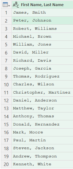
Dealing with First, Last name
Let say we have the above dataset loaded into Power Query Editor. We want to achieve the following tasks by using Column From Examples:
Get the First Name
Get the Last Name
Swap First Name Last Name and remove comma
Super typical. Let’s see how this can be done in Power Query.
We are given a simple table on the left. We need to add three additional columns based on the prefix of the StoreID, and the sales values. The table on the right is the expected outcome.
And here’s the logic:
IF function would probably be the top-of-mind solution. IF is a common function in Excel. It’s widely used for adding conditional columns. Nevertheless, such task is super easy with Power Query as user can achieve it via user interface in Power Query Editor. No formula writing at all. 😉
The challenge – How many transactions with just Brand A and B together?
In my previous post / video, I solved this problem with Power Query. If you are using #Excel 365, did you know you can solve this problem with formula in a helper column? What we want to achieve is to create a flag for each transaction indicating which brands are present in the transaction. The screenshot below demonstrates what we want to achieve. (Please read previous post to understand more about the challenge.)
Honestly, if I am not using #Excel 365, I would not do this with formula as it is too challenging. Nevertheless, with the amazing new functions and dynamic array in #Excel 365, this can be accomplished with a formula as simple as this:
Disclosure: The author earns a small amount of commission (at no additional cost to you) for the product/service successfully sold through the links of [Affiliate].
Wanna buy me a drink!?
Click below photo to my PayPal.Me
I appreciate it. :)