
It’s a common task to split text into columns in Excel. We can do that with “Text to Columns” under Data tab. That’s very handy, however it returns only static result (good for one off task) and could not split text into rows.
With the new function “TEXTSPLIT” in Excel 365 (or latest version of Excel), we can overcome these two limitations with ease.
I will show you the common use cases for this function in the video.
I hope you like this video. If you do, please give a thumbs up, share and subscribe to my channel. 😉
If you prefer reading to wach, please continue to read. Moreover, I will walk you through with examples how to use the optional agruments for this function.
You may download a sample workbook to follow along.
The syntax, as its most basic form, is simple:
=TEXTSPLIT(text, col_delimiter, [row_delimiter], [ignore_empty], [match_mode], [pad_with])
Only the first two arguments are required in most cases. Let’s see what they mean:
- text, the text to be split.
- col_delimiter, the delimiter (could be punctuation marks or texts) that sets the position to spill the text across columns.
- [row_delimiter], it is the delimiter that sets the position to spill the text down to rows. This agrument is enclosed by [ ], meaning it is optional… This is true only when we have the col_delimiter input. When the col_delimiter is skipped, this argument becomes required, otherwise Excel returns #VALUE!
- [ignore_empty], this is optional. By default, it’s set to FALSE, meaning Excel returns a blank cell when two consecutive delimiters are found.
- [match_mode], this is optional. By default, it’s set to 0, meaning Excel performs case-sensitive search for the delimiter. When it is set to 1, Excel performns case-insensitive search. Only applicable when the delimiter is a letter.
- [pad_with], this is optional. The value with which to pad the result. The default is #N/A. This one can be better explained with illustration. 😅
Let’s deep dive by example.
Split into columns
Say we have the text to be split in B3. There is only one delimiter – “,” (comma without space).
Note: If there is space(s) after the delimiter, do include the space(s) within the double quote! i.e. ", " instead of ","
The formula to split the contents into columns is as simple as:
=TEXTSPLIT(B3,",")

Split into rows
To split the contents down to rows, we simply leave the second argument empty, and put the delimiter “,” into the thrid argument.
=TEXTSPLIT(B3, ,",")

Can’t be simplier!
Split into table when we have two delimiters – The WOW moment!
Now we have a text string with two delimiters. The pattern is
A,B;C,D;E,F;G,H
In words, we want to split the contents into a 2-D table. Comma marks the position to split across columns while semi-colon marks the position to split down the rows.
Such task is super complicating without TEXTSPLIT. With TEXTSPLIT, it is piece of cake.
=TEXTSPLIT(B3,",",";")
where comma is the column delimiter; semi-colon is the row delimiter

Isn’t it easy and straight forward?
Dealing with multiple delimiters
In some cases, we want to split the text whenever we see certain delimiters, e.g. we want to treat both comma and semi–colon as the same. This can be achieve by wrapping them into { }.
=TEXTSPLIT(B3, {",",";"})   'to split across columns
=TEXTSPLIT(B3, , {";",","}) 'to split down the rows
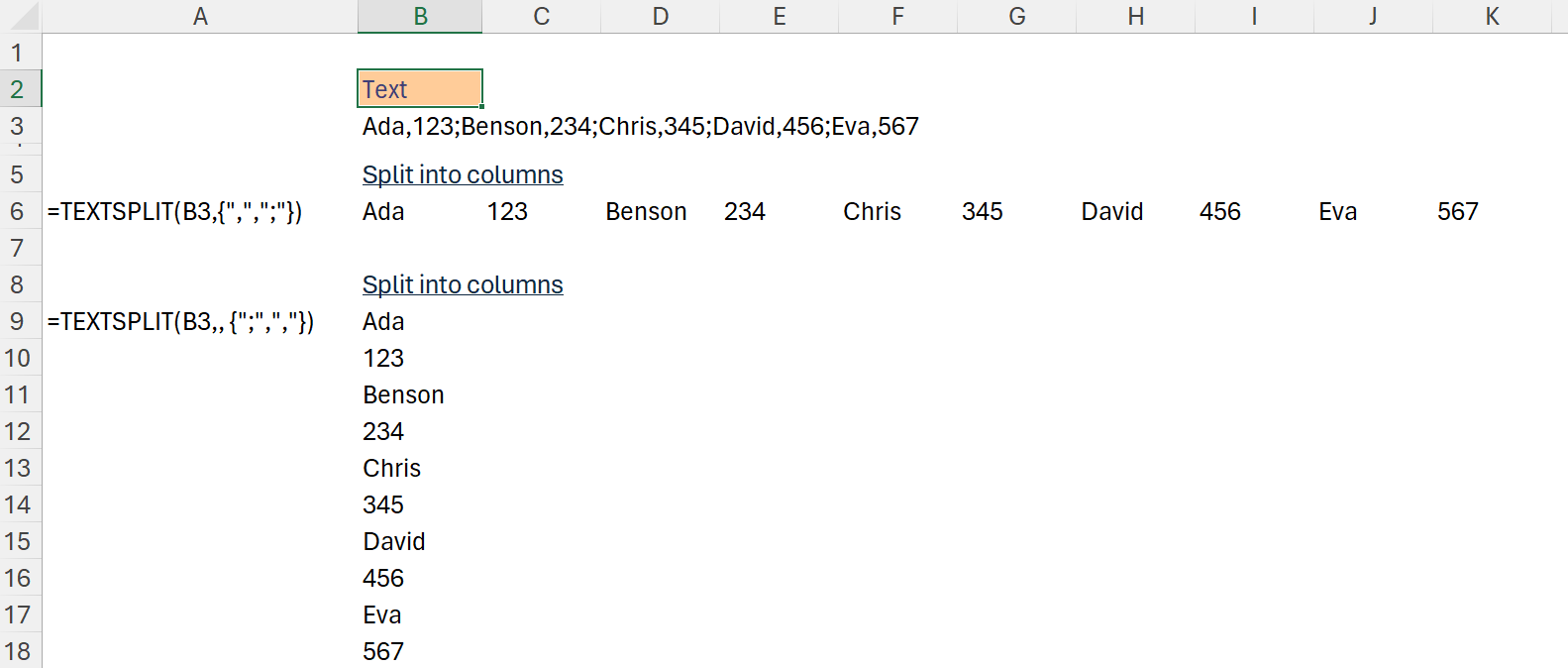
Did you see that the sequence of the delimiters wrapped in the { } does not really matter?
The forth argument – ignore empty
When we have consecutive delimiters, i.e. no text inbetween the delimiter, Excel returns blank cell by default, so that we are aware of the “empty” in the text string. If we don’t want to see blank cells as a result, we can set the forth argument into TRUE. See below:

The fifth argument – match mode
In some scenarios, the delimiter could be a letter instead of punuctation mark. If that’s the caes, we need to be specific if we want to treat “a” as “A” or not? In other words, do we want Excel to perform case-sensitive or case-insensitive search. This is where the fifth argument comes into the play.

The sixth argument – pad with
This argument is applicable when we are splitting text with two delimiters into table.
If we are splitting the text into just rows or columns, we won’t see any impact on the result. See row 6 in the screenshot below.

However when we try to split text into a (2-D) table, there may be chance that the texts won’t fill up all the cells in the resulting (2-D) table. See below:

=TEXTSPLIT(B3, " ", "." , , ,"")
'this is the fommula. With space as column delimiter; dot as row delimiter.  An empty string is input in the sixth argument.  By default, it's #N/A.
To visulize the effect, we put “text” in the final argument
=TEXTSPLIT(B3," ",".",,,"test")
'See the result in row 10 in the screenshot below
In words, pad_with fills in the blank cells in the resulting 2-D table with the text you specified.
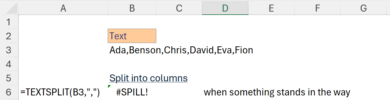
Note: TEXTSPLIT is a dynamic array function that spills the result into multiple cells. Please leave room for the result to spill otherwise you will see #SPILL! error.
TEXTSPLIT is one of the magical functions added to Excel 365. More blogposts about other new functions will come. Stay tune! 😉


