We talked about the new function – TEXTSPLIT in the previous post. Let’s share a use case of myself in this post.
From time to time, I receive email with a long list of recipents. Occassionally, I may want to see who are in the list. The quick way is to copy the list from Outlook and paste it in Excel. When I do that, I end up with a list of Names and Email addresses in a single cell like this:

Fung Wong <FungWong@abc.com>; Ernest <ernestwong@abc.com>; bee <bee@abc.com>; Cat KY Leung <cat.ky.leung@abc.com>; Gary Sou <ahsou@abc.com>; Henry Fong <fymhenry@abc.com>; Mad Lei <mad@abc.com>; Vienna Ng <ViennaNg@abc.com>; Ben Wong <wong@abc.com>; Cat Leung <cat.leung@abc.com>; Francis Lo <francislo@abc.com>; Jacqueline Liu <jacliu@abc.com>; Jim Coral <ahjimmail@abc.com>; Jia MI <jia.mi@abc.com>; Kit Yeung <kit@abc.com>; Kwong Cora <cora@abc.com>; Lo Karen <karenlo@abc.com>
But what I want is something like this:

Before the new dynamic array functions in Excel 365, I can achieve this by a couple of techniques like Text to Columns, Copy and Paste Transpose, Flash Fill. Sound like tedious but it could be done in a minute indeed. Here’s a video I made a couple of years ago when dynamic array functions were not born.
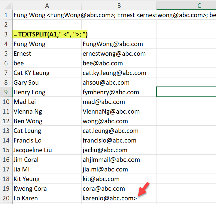
Now, with Excel 365, you won’t believe how easy it could be to perform such task. If you accept imperfection, the solution is as simple as:
= TEXTSPLIT(A1," <", ">; ")
'note the leading and trailing space.

For details of the syntax, please read this post.
The imperfection I mentioned are
- Lack of headers (which could be easily added manually on top, but also could be built into the formula)
- The “<” displayed on the last record (have to deal with it in the formulap)
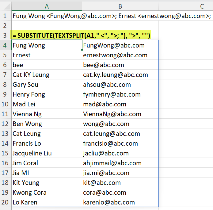
The “>” was kept there as a result of the fact that it is not part of the column delimiter, which is “>; “. To get rid of “>” from the result, we can simply wrap the formula with SUBSTITUTE, like below:
= SUBSTITUTE( TEXTSPLIT(A1," <", ">; "), ">", "")

Want to learn more about SUBSTITUTE, please read this post.
Pretty simple, isn’t it? 😉😉
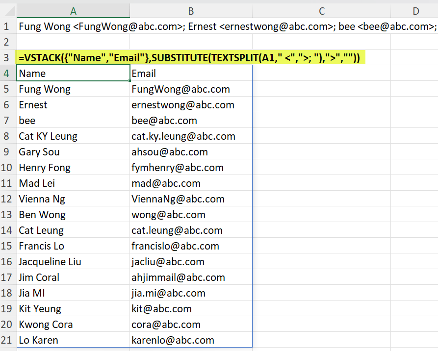
One step further, we can incorporate the headers into the result too.
With another wonderful function VSTACK, it can be done with ease:
=VSTACK({"Name","Email"},SUBSTITUTE(TEXTSPLIT(A1," <",">; "),">",""))

'Note: the use of {} is required in the first argument in this example

What VSTACK does is to stack different arrays together vertically, in the order presented in the function. {“Name”,”Email”} is the construction of an array with one row and two columns.
The new dynamic array functions open a lot of possibilities in simplifying complex formula writing in the past.
You may download a sample workbook to follow along.


