The challenge – How many transactions with just Brand A and B together?

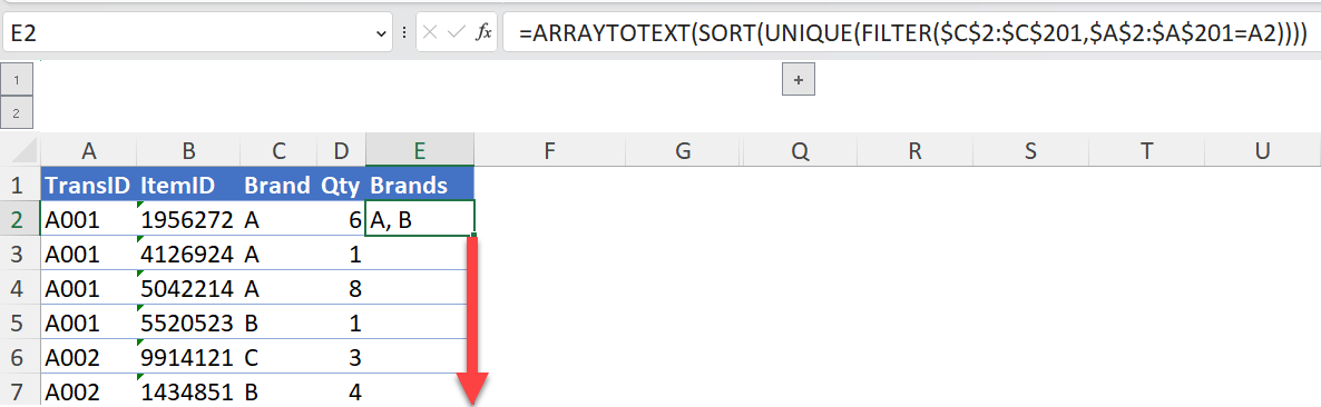
In my previous post / video, I solved this problem with Power Query. If you are using #Excel 365, did you know you can solve this problem with formula in a helper column? What we want to achieve is to create a flag for each transaction indicating which brands are present in the transaction. The screenshot below demonstrates what we want to achieve. (Please read previous post to understand more about the challenge.)

Honestly, if I am not using #Excel 365, I would not do this with formula as it is too challenging. Nevertheless, with the amazing new functions and dynamic array in #Excel 365, this can be accomplished with a formula as simple as this:

=ARRAYTOTEXT(SORT(UNIQUE(FILTER($C$2:$C$201,$A$2:$A$201=A2))))

'where C2:C201 is the range holding the brand of item; A2:A201 is the range holding transaction number

In the following video, I will show you step by step what they do.

You may download a sample file to follow along.

Let’s watch it in action:

If you prefer reading to watching, please continue to read.

Let’s explore the formula inside out.

Step 1 – Get a list of all brands in a transaction

FILTER($C$2:$C$201,$A$2:$A$201=A2)

Remember our task? To identify what brands are bought in a transaction. Since one transaction may have multiple lines, we need a function to scan through the column holding transaction number and return all brands found for the same transaction. FILTER does the perfect job here.

The syntax

=FILTER (array,include,[if_empty])

FILTER takes two required arguments. The first argument is the array (range) we want to filter; the second argument sets the condition(s) to filter.

In our example, the formula is:

FILTER($C$2:$C$201,$A$2:$A$201=A2)

It instructs Excel to filter the range C2:C201 (i.e. the Brand) where the transaction numbers in the range of A2:A201 are equal to the transaction number of current row. In plain English, please give me all the brands you found with the same transaction number of the current record in the dataset.

And Excel returns this as a result:

See, it returns an array of {“A”; “A”; “A”; “B”} as there are four lines for transaction A001. Note: Traditional Excel won’t give you an array that spills over to more than one cells (Unless you specify the exact size of the array to be returned by pressing CTRL+SHIFT+ENTER, aka array formula). However, with Excel 365 (since the introduction of Dynamic Arrays), Excel can return an array as a result. This behavior is called spilling.

Step 2 – Remove duplicates aks get a unique list of brands

WOW! That’s great. But I don’t need “A” to be present three times. What I need is a unique list of brands. Yes…. you just called it out! The UNIQUE function. It returns a list of unique values in a list or range.

The syntax:

=UNIQUE(array,[by_col],[exactly_once])

In our example,

UNIQUE(FILTER($C$2:$C$201,$A$2:$A$201=A2)) returns

UNIQUE({"A"; "A"; "A"; "B"}) returns

{"A"; "B"} as a result

The result:

Step 3 – Sort the list in ascending order

This step is subtle but important. Let’s look at transaction “A009”. In the transaction, Brand B was input before Brand A. As a result, the formula returns an array of {“B”; “A”} instead.

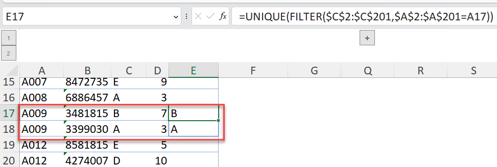
This is not ideal as we don’t want to treat {“A”; “B”} as different from {“B”; “A”}. In basket analysis, what we want to know is if a transaction contains both brands “A” and “B”, the sequence does not matter.

By wrapping the result returned in Step 2 by SORT function, which sorts the contents of a range or array, we eliminate the impact of sequence.

The syntax:

=SORT(array,[sort_index],[sort_order],[by_col])

The formula:

SORT(UNIQUE(FILTER($C$2:$C$201,$A$2:$A$201=A2)))

The result:

Step 4 – Put the array into a single cell, so that we can fill the column

We don’t want the result to be spilled across multiple cells. Instead, we want it in a single cell, with comma separated. ARRAYTOTEXT does it nicely in this scenario.

The syntax:

ARRAYTOTEXT(array, [format])

The formula:

=ARRAYTOTEXT(SORT(UNIQUE(FILTER($C$2:$C$201,$A$2:$A$201=A2)))) 

The result:

Still remember our task? We need to create a helper column to indicate all brands involved in a transaction. That’s why we need a single-cell result so that we can copy it down to fill up the entire helper column.

With the helper column set up, we have the fundament element to filter transactions of both brands “A” and “B” only, or any other combination of brands, with ease!

Extra: Don’t miss the Bonus section in my video. I take a step further to bring the analysis into a more dynamic way. 😎

What do you think? Do you feel the power of dynamic arrays and the new Excel functions? Please leave your comments below.