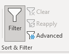
Did you notice that there is a “Reapply” button next to Filter on the Data Tab of ribbon? And wondering what it does? 🤔

Indeed, the “Reapply” button is dim until you have applied filter to at least one column.

To illustrate how to “Reapply” filter, let’s start with a simple example.

Situation

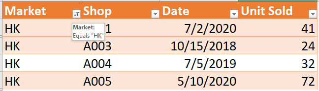
We have applied a filter on Market to show records of “HK” only, as shown below:

Then we realized that the Shop “A004” should belong to “SG” market, so we revise the data on the spot…

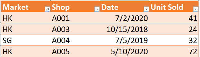
However, filter is not dynamic. In order to filter out the record of A004, which we have just revised it to SG Market, we have to reapply the filter again.

(If you are using Excel 365 and want to have dynamic filter, check out the new FILTER function)

Here comes the “Reapply” button to rescue!

As simple as this. 😉

You may be thinking… it requires two clicks (first click on Data; second click on Reapply). Why don’t we simply set the filter from the filter pull down? It takes two clicks only too.

Well… you are absolutely right when you are only dealing with one column. What if when we have filters set on multiple columns? The number of clicks would be a multiplication of 2 and the number of columns with filter set. That makes the difference. Right?

Having said that, if two-clicks is a concern to you, let’s use the keyboard shortcut:

Ctrl+Alt+L

How do I know this shortcut? Excel told me. 😁

Excel shows tips in subtle way… what Excel needs from us is our attention!