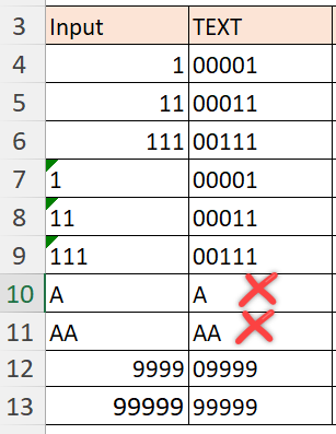
Pad a column to fixed length with #Excel formula

Here’s the situation: We have a column of values with various lengths, from 1 to 5 letters. We want to convert that into a fixed length of, say 5 letters, padding with zero(s). The following screenshot illustrates the requirement.

How would you do it? If “IF” is on top of your mind, please continue to read as I am going to show you a few diverse ways to achieve this. The approaches I am going to show you are:

Using TEXT (works best when we have numeric values only)
Using nested IF (probably the most commonly used approach, but not necessarily the best)
Using SWITCH (an alternative to nested IF, more readable and easier to construct)
Using LET (to solve the problem step by step; and make the formula more readable)
Using basic functions and logic (this is what I recommend)

Note: SWITCH and LET are available in Excel 365

You may download a sample file to follow along:

sample-workbook-pad-text-into-fixed-length.xlsx Download

I assume you understand the basics of these functions: IF, TEXT, REPT, LEN. If you don’t, please review them first.

Let’s watch it in action:

If you prefer reading to watching, please continue to read.

Using TEXT

The formula is quite easy.

=TEXT(A4,"00000")

A better variation is:
=TEXT(A4,REPT("0",$H$1))

where A4 resides the value to be padded with 0; H1 resides the number of the letters we want

I discussed this topic before. Please review this post if you want to learn more.

I added a twist of using REPT here to make the solution more dynamic. REPT takes two arguments: The “Text” and the number we want to repeat it. So REPT(“0”, $H$1) returns a text string of “00000” in the above example; and it responds to the number we input in H1.

Although it is a simple solution, it does not work when we have non-numeric values involved:

Using nested IF

When we deal with different scenarios, it is quite common to think about writing an IF statement to cater to different scenarios. For this problem, we would first identify the length of the text. If it contains one character, then we pad it with four leading zeros; if it contains two characters, then we pad it with three leading zeros; if it contains three characters, then we pad it with two leading zeros; if it contains four characters, then we pad it with one leading zero; else we just take the text-form of it.

To translate the above into Excel formula, we have:

=IF(LEN(A4)=1, "0000"&A4, IF(LEN(A4)=2, "000"&A4, IF(LEN(A4)=3,"00"&A4, IF(LEN(A4)=4,"0"&A4,TRIM(A4)))))

Tip: The TRIM function in the last argument is used to ensure all results returned with be text

This formula works. However, it is not easy to construct nor easy to read. Another drawback of this approach is the difficulty in modification. Think about this, what if the requirement now changes to a fixed length of 9? OMG… how many IF we need to nest in the formula. 😰

Of course, we may apply the trick of using REPT to make it more dynamic. Nevertheless, I would not do so here as I don’t want to show you a monster formula. We will see how we can incorporate that part later.

Using SWITCH

SWITCH may be a new function to you, but it is easy to understand with example. Just look at the below and try to understand it.

=SWITCH(
LEN(A4),
1,"0000"&A4,
2,"000"&A4,
3,"00"&A4,
4,"0"&A4,
5,TRIM(A4),
"out of range"
)

Need some help? The comments below after // explains what it does

=SWITCH(
LEN(A4), //the expression we want, it returns the length of the text in A4
1,"0000"&A4, //when the expression returns 1, pad the text with "0000"
2,"000"&A4,  //when the expression returns 2, pad the text with "000"
3,"00"&A4,   //when the expression returns 3, pad the text with "00"
4,"0"&A4,    //when the expression returns 4, pad the text with "0"
5,TRIM(A4),  //when the expression returns 5, TRIM the text
"out of range" //else, returns "out of range"
)

Is it much better than the nested IF approach? Having said that, it shares the same drawback: Need to modify the formula when the number of fixed length changes. Even though it’s easier (than nested IF) to add further options in this approach, it’s not ideal.

Using LET

LET is a super helpful function (in Excel 365) to construct complicated formulas. It helps break the complexity into simple bit-size logical steps.

Think about this simple example:

Let x be 1, y be 2, x+y = 3

Now we can simulate this in Excel formula and the construction is very intuitive.

=LET(  //let
x, 1,  //x be 1
y, 2,  //y be 2
x+y    //return x+y
)

Isn’t it intuitive? 😎

Let’s apply it to solve our problem

=LET(
n, LEN(A4),
target, $H$1,
gap, target - n,
pad, REPT("0", gap),
pad & A4)

In plain English, let

n be the length of the text in A4
target be the fixed length specified in $H$1 (note: it’s absolute reference as we plan to copy the formula down)
gap be the number of zeros required to pad (defined by target minus n)
pad be the padding string (defined by repeating the number of zeros stated in the previous step)
return the result as pad & the text in A4

That’s it!

This formula helps walk your user through your thinking logic. Not only does it improve readability but also it improves performance as most steps get evaluated once.

LEN(A4) got evaluated only once in this approach but multiple times in the nested IF approach.

And the best part is, this formula is truly dynamic. It works like a charm even when we change the number in H1! Watch this:

Isn’t it cool? 😎

What? You don’t have Excel 365? I heard that. Here’s come the final solution that works in all versions of Excel.

Back to Basic

Let’s start with the static approach, i.e. a fixed length of five is required. The formula is as simple as the following:

= RIGHT("00000" & A4, 5)

Yes. It is! And it works!

Wondering why? A picture tells a thousand words:

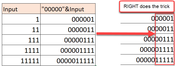
Using this approach, we don’t need to care about the length of the text. We padded it with five zeros “00000” anyway, followed by extracting the five letters in the right. Make sense? 😉

To make it responsive to the number input in a cell (H1), we just need a twist:

Static:
= RIGHT("00000" & A4, 5)

Dynamic:
= RIGHT(REPT("0",$H$1) & A4, $H$1)

Note: Using this approach, you have to make sure your source data will not have any value with length that is larger than the number input!

Tell you a secret. In my early stage of using Excel, I thought that the longer the formula I could write to solve a problem, the better the Excel skill I possessed. Now, I am a fan of simplicity.

Do you have other formula approach to solve this problem? Please share with us by leaving a comment. 🙌