by hiding all unwanted columns and rows

Did you know there are 16384 columns and 1048576 rows on a worksheet? We have the flexibility to navigate any cells within this large range! Nevertheless, this is NOT what we want some time. Think about when you have created a wonderful report or dashboard, you want your audiences to stay focus on the range with information. A simple way to achieve this is to hide all unwanted columns and rows.

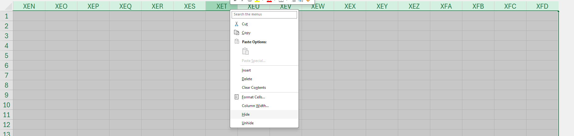
To hide unwanted columns

1. Click the header of column I (in the example above; it’s totally up to you where to start with)
2. Ctrl+Shift+Right arrow (to select all the columns on the right)
3. Left click a column header -> Hide (Shortcut: Ctrl+0)

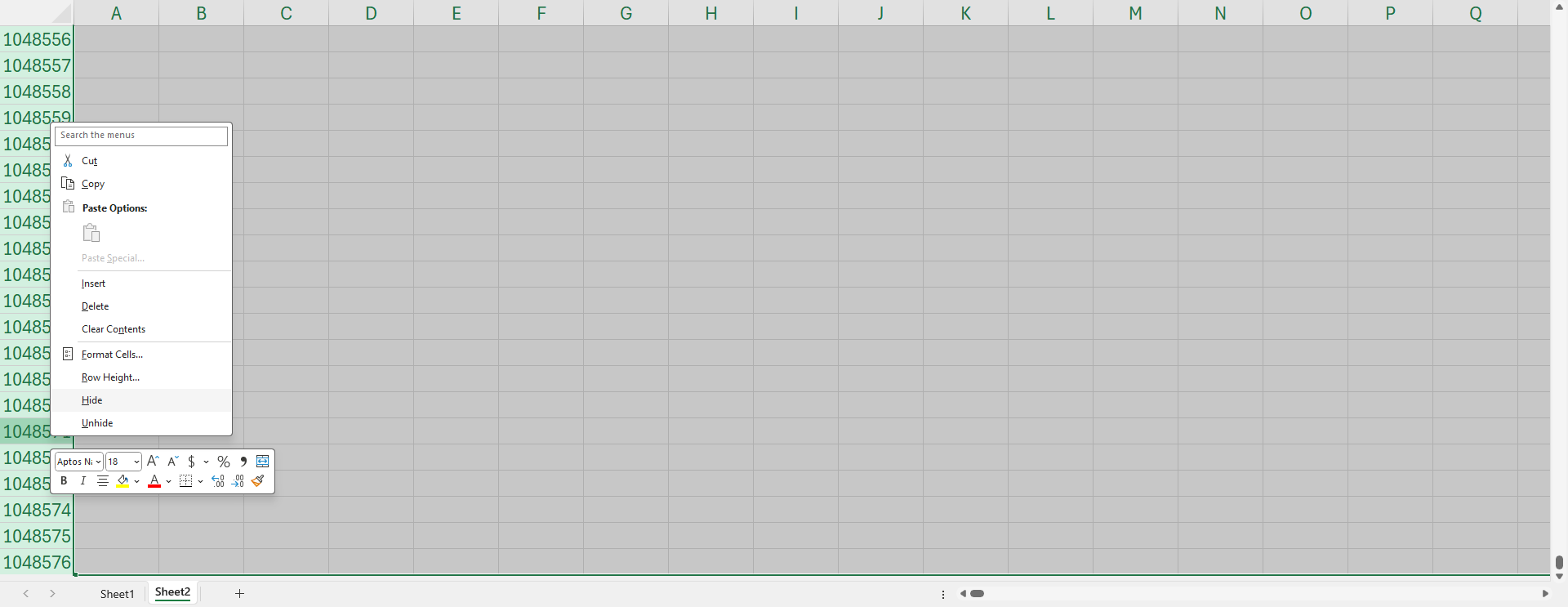
To hide unwanted rows

1. Click the header of row 23 (in the example above; it’s totally up to you where to start with)
2. Ctrl+Shift+Down arrow (to select all the rows below)
3. Left click a row header -> Hide (Shortcut: Ctrl+9)

Here we go! Your have successfully removed noises from your worksheet and let your audiences stay focus!

As simple as this! 😎