Quite a long time ago, I wrote about two different approaches of preparing dependent dropdown menu in Excel. The first approach was for non Excel365 users, while the second approach was for Excel365 users. You may refer to the post here.

In this post, I will be using the same sample workbook, solving the same problem, but by a third approach using OFFSET, an Excel function that went unnoticed. 😅

You may wonder why? Because of the limitations of the first two approaches:

For the first approach using INDIRECT function, it’s quite flexible indeed.

For example, if we have four items in the first down drop menu, then we must prepare five different tables as shown in the screenshot above. You can imagine, it may take some time to prepare the tables required when we have a super long list of items using this approach. In short, the setup process would be a major hurdle using this approach, when there is a long list of items.

For the second approach using dynamic arrays, I would say that’s very easy to setup. However, as of the date this post is written on, Data Validation does not accept input of formula using dynamic array functions such as FILTER. It means, we have to rely on helper columns (What you see in column I and beyond in the screenshot below).

This limitation makes the dependent dropdown menu NOT automatically expand with Excel Table. We need to copy down formula in column I in respond to row addition to the input table. Although not a big effort, it’s just not good enough.

By using the third approach using OFFSET function, I can bypass the hurdle of the first approach, while enjoying the simple table setup:

The challenge of this approach is probably you need to feel comfortable in writing formula like this:

=OFFSET(tb_Menu[[#Headers],[Item]],MATCH(H3,tb_Menu[Course],0),,COUNTIF(tb_Menu[Course],H3))

And also you need to know how to convert it into a Named Range.

IMPORTANT: Pay attention to the relative cell reference H3 in the above formula . When this formula is input in the name manager dialog box, the active cell has to be in I3. This means, H3 refers to the cell that is one cell to the left of the active cell. This is critical for this to work properly.

If you want to study the details later, simply download the sample workbook, modify the contents in the table and use it.

If you want to understand how it works, its major limitation, and extra tip to make sure it works on any worksheets, please see detailed explanation below.

Convert your dataset into Excel Table

For efficiency, convert the range of data into Excel Table first!

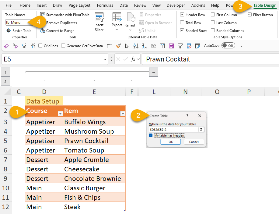
1. Select the range D2:E13 (in above example) -> Insert -> Table (Shortcut: CTRL+T)
2. Check the box “My table has headers” (unless you range of data does not have headers), then OK
3. Go to the tab “Table Design”
4. Give it a meaningful name

Setting up the first dropdown menu

For simplicity, UNIQUE function is used for the content for the first dropdown menu. In cell G3, input this formula

=SORT(UNIQUE(tb_Menu[Course]))
'Note 1: SORT is optional
'Note 2: Since we are referencing an Excel table, the structural referencing "tb_Menu[Course]" is automatically input for you when you select the column of "Course" (See below)

If you are not using Excel 365, you probably do not have the UNIQUE function. If that's the case, please input the unique list manually.

Now we have the list of “Course” for the first dropdown. Let’s do it with Data Validation:

If you are not familize with the steps for the above, please refer to the post here.

Setting up the dependent dropdown

Before we start, let’s walk through the high-level idea first.

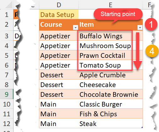
We are expecting a “dynamic” dependent dropdown menu. In our example, it depends on the “Course” we input. There are three potential values: “Appetizer”, “Dessert” and “Main”. 

When “Appetizer” is input, we would expect the dependent dropdown to display “Buffalo Wings”, “Mushroom Soup”, “Prawn Cocktail” and “Tomato Soup”. In other words, we expect the four items starting from the first item in the list!

For the same token, when “Dessert” is selected, we expect the three items starting from the fifth item; when “Main” is selected, we expect the three items starting from the eighth item in the list.

OFFSET is here to help! 

What it does? In short, it returns a range (could be a single cell, a one-way table, or a two-way table) based on the location and size you specified.

The syntax is:

OFFSET(reference, rows, cols, [height], [width])

• reference is the starting point (can be a cell or a range);
• rows is the number of rows to go down (or up) from the starting point;
• cols is the number of columns to go to the right (or left) from the starting point;
• height is the size of the range in number of rows you want to return (when omitted, it is the size of the reference);
• width is the size of the range in number of columns you want to return (when omitted, it is the size of the reference)

You may refer to this post from MS Support for details.

To give an example in plain English, if I want to return the list of items for Appetizer, I need Excel to go to cell E2 (reference), go down by 1 row (rows), stay on the same column (cols), and then take the 4 cells below (height) in the same column (width).

To translate it into formula, it is:

=OFFSET(E2,1,0,4)
Tip: the "0" can be omitted

For the same token, the formula to grab the list of Dessert can be written as

=OFFSET(tb_Menu[[#Headers],[Item]],5,,3)
Note: As we are referencing to an Excel Table, the above structural reference will be written for you automatically when you point to cell E2

As you can see, the first argument “reference” (starting point) and the third argument “cols” are static while the second argument “rows” and the forth argument “height” can be changing, depends on what item we need based on the first input. In other words, if we can make these two arguments dynamic, depending on the input to the cell on the left, then we are one step closer to our goal.

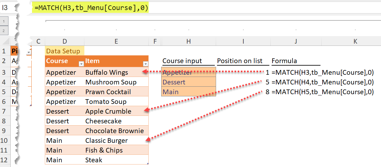
Making the “rows” dynamic using MATCH

To get the number of rows to go down (rows), we can apply the following formula

=MATCH(H3,tb_Menu[Course],0)

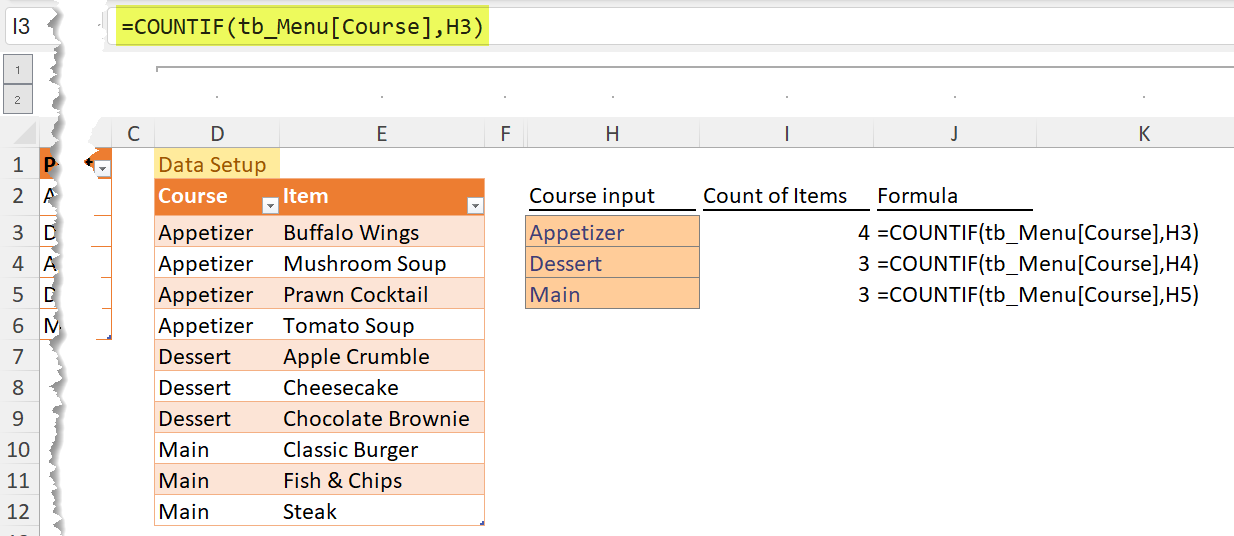
Making the “height” dynamic using COUNTIF

To get the number of rows to be included (height), we can apply the following formula

=COUNTIF(tb_Menu[Course],H3)

So far so good, right?!

To substitute these two formula into the OFFSET function, we have:

=OFFSET(tb_Menu[[#Headers],[Item]],MATCH(H3,tb_Menu[Course],0),,COUNTIF(tb_Menu[Course],H3))

This formula returns a dynamic array based on the input in H3. Yeah!

Now, you probably think that the next step is straight forward… simply copy the formula for Data Validation. If we do so, we will get the following error!

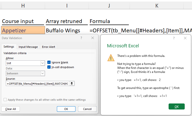
By reading the error content, I thought it is not allowed to input formula as the source for list in data validation. Of course it is not (100%) true. We can input a formula start with “=” sign, we just need a little twist.

Creating a dynamic Named Range

Let’s copy this formula first

=OFFSET(tb_Menu[[#Headers],[Item]],MATCH(H3,tb_Menu[Course],0),,COUNTIF(tb_Menu[Course],H3))

'Reminder: H3 is a relative cell reference. Make sure your active cell is I3 (i.e. the cell to the right of it)

then

1. Go to Formula tab
2. Go to Name Manager
3. Click “New…”
4. Give it a meaningful name, e.g. “Dropdown” 😅
5. Paste the formula into the “Refers to:” (don’t forget the equal sign)

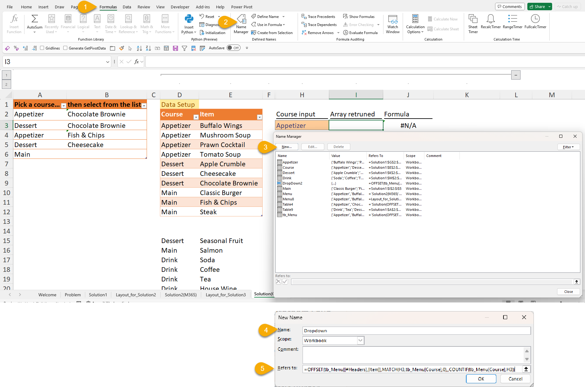
After clicking OK, you will see the following. 

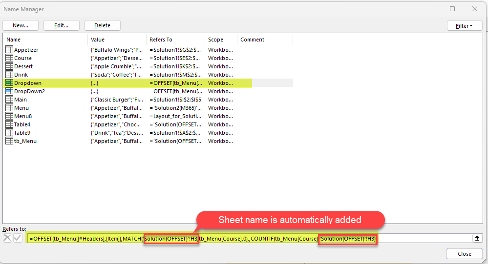
Did you see that? The sheet name is added to the cell reference automatically. If you are planning to use the dependent dropdown menu only on the worksheet you create this, it’s totally fine to accept this by clicking “Close”. 

Let’s click “Close” to accept it for the moment. We will come back to this at the end.

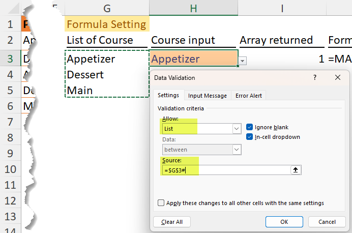
Setting up the Data Valdiation

Now we have set up the Named Range called “Dropdown” using the OFFSET function, we can put it into the data validation as shown below:

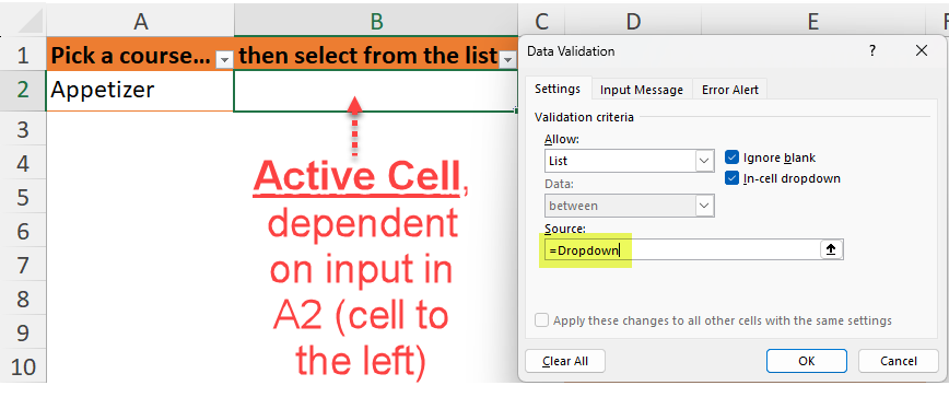
It is critical to pay EXTRA ATTENTION to the location of the active cell when you apply this step. What we set up in the Name Range is based on the input in the cell that is to the left of the active cell, we have to make sure that the first input that determines the content of the dynamic list should be residing one cell to the left of the active cell. In our example above, the input of “Course” resides in cell A2, and the active cell that we apply this Named Range is B2. THIS IS SUPER IMPORTANT!

When we have all these set up properly, you can expect the following:

Please note the following:

1. Range A1:B2 had been converted into Table before applying the data validation
2. Data validation on A2 had been applied using the technique described in the section “Setting up the first dropdown menu” above

Tip: To expand the Table when reaching the end (lowest right cell) of the table, press Tab

Now we have created a dynamic dependent dropdown menu within Excel Table, without the hassle of setting up too many tables. Isn’t it cool? 😎

Limitation

Having said, there is one major limitation of this approach. When new data comes in, like this:

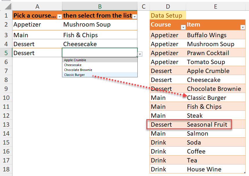
You would not expect to see “Classic Burger” as “Dessert”. It does because the new data breaks the logic of the formula created, that requires all “Course” of same type be grouped together. 

Lucikly the fix is easy: simply sort the first column after new data comes in!

BONUS – Make this dependent work on other sheets!

Still remember this?

The automatically added sheet name at this step make the dependend dropdown works properly only on the same sheet. It is because the formula will always look into the cell that is left to the active cell of the worksheet “Solution(OFFSET)”.

If we want to make this formula work for “current” worksheet, we have to remove the sheet name BUT keeping the ! (exclaimation mark).

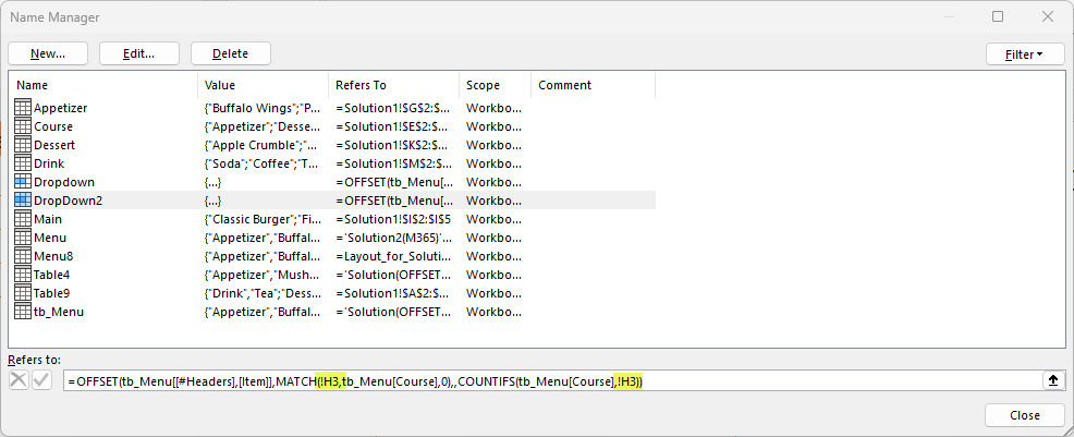
You may refer to the “DropDown2” in the sample workbook. Try to apply both Named Ranges to see the difference.

I hope you find it useful. Please leave your comments on what you think about it! 😉