…with and without Dynamic Arrays (which is available to Microsoft 365 users only)

Got a question from a friend recently:

Is it possible to show a different set of questions in a dropdown list depending on the answer input from a previous question using Excel?

Me:

Of course! It is just a dependent dropdown list using Data Validation.

I had blogged about the technique for different scenarios. However I have not yet written a post for the basic of it. So, let’s do it. 😁

What is dependent dropdown?

A GIF tells thousand words:

It is clear, isn’t it?

Then the question is how?

There are many different ways to achieve this because it is Excel. Instead of showing you many different ways, I am going to focus on two approaches. One is for majority of Excel users who are not accessible to Dynamic Arrays (Microsoft 365); and one for Microsoft 365 users.

You may download a sample file to follow alone.

Indeed, you will find that it is easy to deploy as long as you have the data setup properly.

Scenario

Using our example showed above, we want user to input a course (from a list) first. Then a dependent list of item will show up for selection, according to the item that has been selected before. In order to achieve this, we need some preparation works.

Data Setup (NON-Microsoft 365 approach)

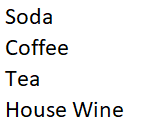
First, we need to define the list of courses for selection; followed by the list of item for each course. Then turn the lists into Excel Tables. (Don’t know how? Pls check it out HERE!)

Here’s the successful factor:

We have to rename the dependent tables properly.

As shown above, Table 2 to 4 are named as “Appetizer“, “Main” and “Dessert” respectively. The names have to be exactly the same as the items available for “Course”. When we have this setup properly, the rest will follow logically. Please note we have also renamed the Table1 to “Course” as a good practice.

Setting up the 1st (Independent) dropdown list

1. Select the range (A2:A4 in our example) where you want user to input Course
2. Go to Data tab
3. Click Data Validation
4. Select List from the dropdown for “Allow” (Tip: Ensure the “In-cell dropdown” is checked”)
5. Input the following formula as the “Source:”
   =INDIRECT(“Course”)
6. OK

Note: The above set up is not mandatory but highly recommended. Although we may ask user to input the type of course they want directly, manual input could usually lead to unexpected results and hence problems. It’s better for us to (kind of) control what user can input by setting up this data validation first.

If you have followed along so far, you should be able to see the dropdown list available when you select A2, A3 or A4, like below:

Setting up the 2nd (Dependent) dropdown list

This is more or less the same as the steps involved just before. Can you spot the difference in the following screenshot? 😁

Changes are highlighted below:

1. Select the range (B2:B4 in our example) where you want the dependent dropdown list
2. Go to Data tab
3. Click Data Validation
4. Select List from the drop down for “Allow” (Tip: Ensure the “In-cell dropdown” is checked”)
5. Input the following formula as the “Source:”
   =INDIRECT($A2) ‘note: there is no $ for row, i.e. relative row reference
6. OK

Here we go!

The key is the use of INDIRECT. It instructs Excel to look into different tables indirectly, according to the item input in the adjacent cells (A2:A4). Want to learn more about INDIRECT, read the blogpost HERE.

How to update the list?

It is easy. Suppose we want to add items to each course, simply add the new item(s) to the corresponding tables. As shown below:

Wait… What if we need to add a new “Course”, say “Drink” with the following items?

Indeed, it is easy too.

First we add “Drink” to the table “Course”; then we create a new Excel Table called “Drink” as shown below:

This is it.

If you are using Microsoft 365, please continue to read. You will see how Dynamic Arrays could make our Excel life even simpler!

(Note: It’s best to use video, instead of blogpost, to illustrate how dynamic Dynamic Arrays is. A video is under production. Please stay tuned. Until that, please continue to read.) 😉

Data Setup (Microsoft 365 approach)

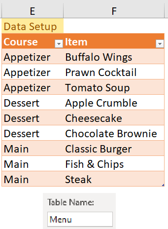
Instead of creating multiple Excel Tables for each list, we can create a single Excel Table with two columns, as shown below:

Then we need two helper formulas as the sources for our data validations.

Formula Setup

In H2, input the following formula:

=UNIQUE(Menu[Course])
'UNIQUE returns a list of unique item from the column "Course" of the Table "Menu".

The result spills automatically. The formula was input into H2, but it spills the results from H2 to wherever needed, or H4 in our example.

When we have the formula set up in H2, we are now ready to create our 1st (Independent) dropdown list.

The steps are more or less the same with only one exception: The formula used in the “Source” of Data Validation.

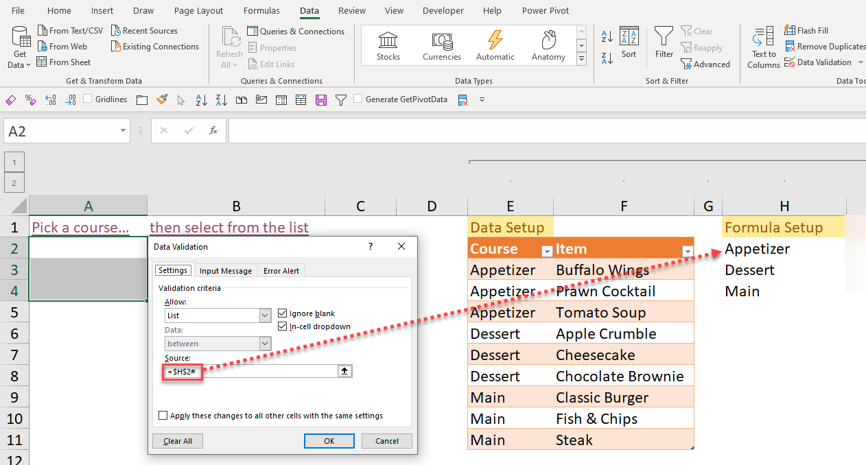
The formula used:

=$H$2#
'Note: Absolute reference is used; and most importantly the # at the end that tells Excel it is a dynamic arrays originated at H2

To make the next step more “visible”, let’s input something from the list in A2:A4 first.

Then we can input the following formula in I2:

=TRANSPOSE(SORT(FILTER(Menu[Item],Menu[Course]=A2)))
'Copy down to where you expect your entry form ends

The function FILTER is the key here. It returns the [Item] in the Menu Table where the [Course] is equal to the input in A2. In short, it returns a dynamic list of items depending on the input in A2.

The use of the function SORT is optional here; it helps to sort the filtered list.

The use of TRANSPOSE is to turn the result from vertical to horizontal, so that we can copy down the formula to wherever needed.

Important notes:

The above formula should be input on the same top row of the entry form. For example, if our input starts from A5, we should input the above formula on a column of row 5 too. Moreover, there should be enough rooms on the right to the column for the results to be spilled. I will explain more in the video. 😅

Now we are ready to set the data validation rule to B2:B4. If you have followed through so far, I guess you probably know what to input as the source…

=$I2# 
'Note: Relative row reference is used as it references to a cell that is relative to row. In other words, we plan to copy the formula down.

Now it’s all set!

The best is yet to come…

It is super easy to add new items or new courses! Watch this:

If you have read all the way down here, I hope you embrace the power of modern Excel as much as I do. Dynamic Arrays is only one of those great features. New functions such as LET, LAMBDA are simply amazing. Not to mention the XLOOKUP. 😎

What do you think? Please share your thoughts by leaving comments below.