In Power Query Editor, there is a button of “Keep Duplicates” in the ribbon. It’s located under Keep Rows in the section of Reduce Rows in the Home tab of the ribbon.
With this, it is super easy to keep duplicates in our dataset. By the way, duplicates mean value appears more than once. Let’s take a look at the screenshot below, “A”, “B”, and “F” are duplicates,
IMPORTANT: Power Query is case sensitive!
while “b”, “C”, “D”, “E” are uniques (i.e. values appear only once).
Unique values appear only once
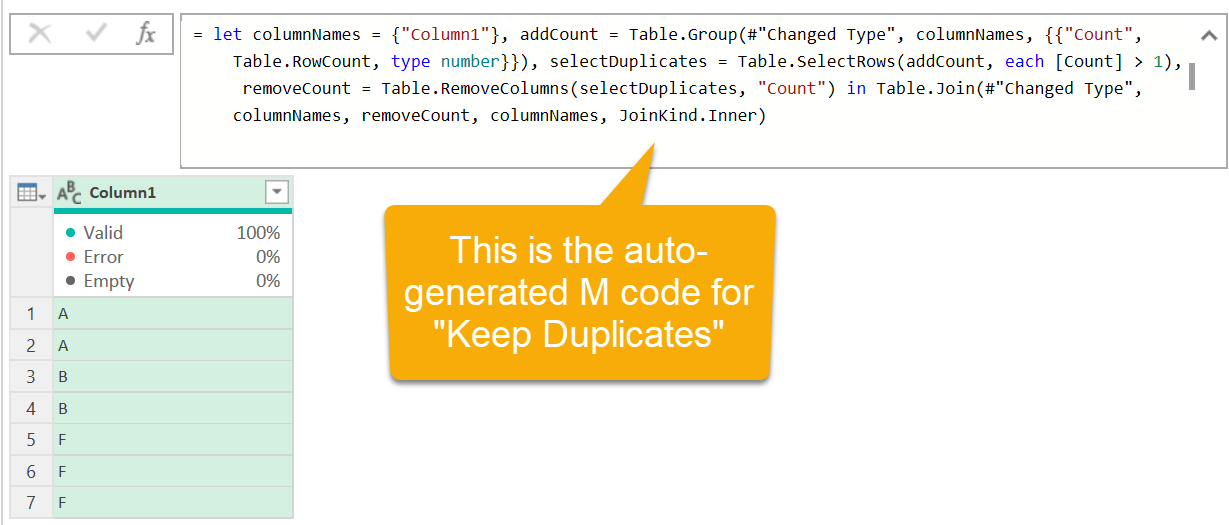
When we apply “Keep Duplicates” to Column1, we obtain the following result.
Keep Duplicates is a result of a quite complicated M code…
The good thing about Power Query is, we do not have to worry about the M code auto-generated. Power Query handles the M codes, we handle the User Interface, which is mainly “select and click”. Easy for users, isn’t it?
When we import data into Power Query editor, we should set the scope of data that we need. That means selecting only the rows and columns required for further processing. In the following video, I will show you different ways of keeping the rows that you need with Power Query.
Let’s think about this scenario. In the first encounter of Power Query, you were presented with demonstrations that show all the powerful transformations done by Power Query. You were surprised and amazed with the demos. Normally we did not pay attention to subtle details about the powerful tools. We jumped straight into all the transformation steps by following examples. Sometimes it works, something it doesn’t. And then you feel frustrated as you don’t know why some calculations give you unexpected results. If this sounds familiarize, I will say, this is because we are all trying to run before walk. 😅
In this blogpost, and in the video, I will talk about a basic but crucial step in Power Query – Data Type.
Data Type in Power Query is NOT formatting in Excel
Formatting does not change underlying values, defining data type in Power Query does.
When we work with data using Power Query, defining data type of each column before loading the result is a best practice. Please don’t mix it up with formatting in Excel. Defining data type to a column is fundamentally different from applying a formatting. In Excel, when we apply a format to a number, the underlying value of the number remains unchanged. On the contrary, when we define data type of a column in Power Query, all the values under the column will be converted to the data type that’s being defined.
Power Query is not behaving like Excel when doing calculation
Nevertheless, defining data type in Power Query is not for data conversion only. We need the data type to be explicitly defined before some calculations happen. Otherwise, we may have unexpected results returned. The worst scenario is we don’t even know that. For example, when you try to add “10” to 10, Excel returns 20 while Power Query returns error. Similarly, when you try to add 10 to an empty cell, Excel return 10 but Power Query returns null. In general, number does not work with text; text does not with number in Power Query.
Close and Load to is the last step in Power Query, but the first step in your reporting process. When I first learned Power Query, I preferred loading the result to Table as I could “see” the result on a worksheet. That’s normal, right?
The more I use Power Query, the more I realize that I rarely load my result to table directly. Most of the time, I load all queries to connection only. This is particularly true when my goal of cleansing/transforming data is for further analysis using Pivot Table (or data modeling).
If your goal is to use the processed data for Pivot Table, load the queries to connection.
In this short video, I will show you how to change the load destination from Table back to Connection only. Also, I will show you why it is better to load the queries to connection only when you are planning to use the result in Pivot Table.
If we want to see when a workbook was last modified, we can see the information from File Explorer,
or Excel Info
Very handy indeed.
However, if you want the information to be put on a worksheet, there is no formula to retrieve that information directly. No worries, we can get that piece of information using Power Query and it will be super easy (if you are not going to rename your workbook nor move it to a new folder). In fact, it is not difficult at all to turn the solution into a dynamic one. Let me show you step by step.
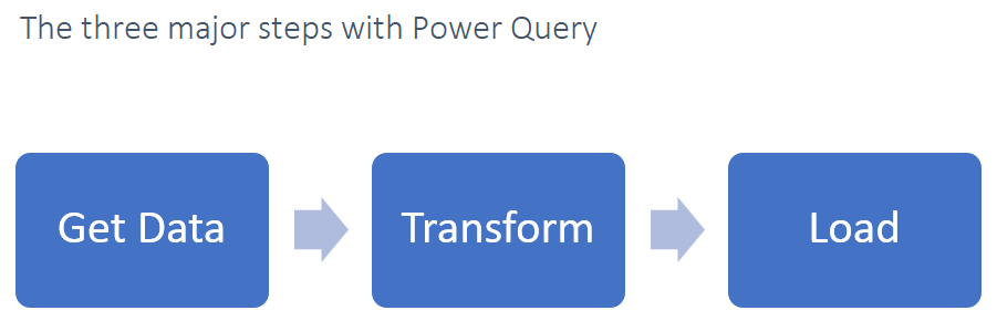
As mentioned in the previous post, the awareness of Power Query is extremely low. In my experience, the hurdle for people who have learned Power Query but not feeling comfortable in using it is the fact that they are not well informed about the three major steps involved:
If we learned Excel long enough, we are all trained to move cells around on worksheets for reshaping data; copy and paste for data consolidation; setting formulas for data cleansing or calculations, and so on and so forth. In Power Query, we are doing the same but through quite a different process, listed above. That is normal for people having difficulty to start with Power Query.
So, from now on, please bear in mind that the first step when using Power Query is always getting the data.
Power Query empowers users to get data from multiple sources. It could be data sitting within current Excel Workbook, another Workbook, CSV/TXT files, Web, PDF, or even files from a folder and many more. One of the cool things in this process is that we don’t even need to open the files with the data we need. Remember this: Power Query can read the data from a file (or source) without “opening” it.
Once we get the data (connect to the data source), all the cleansing / transformation magic will happen within Power Query Editor.
It is particularly important to get ourselves familiarized with the User Interface of Power Query Editor because most of the transformation steps are performed via different command buttons on the ribbon.
To illustrate the process and the User Interface of Power Query Editor, I have made this video:
Cantonese VO is under production.
I hope you like it. If you do, please give it a thumbs up, share and subscribe to my channel.
More videos on Power Query are coming. Stay tuned! 😉
Depends on what? It depends on what you do and how you do it in Excel. 😉
True/False moments
Excel is the core software I use for work
I use Excel for data analysis
I need to deal with data from multiple sources (or from multiple Excel workbooks)
I spent hours cleansing/transforming data before I could start analyzing it
I do repetitive cleansing/transformation tasks on a regular basis
I consolidate data by “copy and paste” data from multiple files
I do most of the data work with VBA
If you answered TRUE to more than two questions, then you should really consider setting Power Query as your learning goal in 2022. Believe it or not, you don’t need one year to learn it before you can use the power of it. Although mastering Power Query could be a long journey, most of us are not required to be at the expert level. (I am not an expert of Power Query either.) Just the basics of Power Query are good enough to change your (work) life.
Let me share a quick tip of Power BI today coz I work with Power BI Desktop a lot recently. 😎
What I am going to share in this post is my favorite shortcut key in Power BI Desktop. Honestly, I know just a few shortcuts in Power BI Desktop (much less when comparing to Excel). Nevertheless, the following shortcut is absolutely my all-time favorite, even a lifesaver! What is it?
Finding and highlighting differences should be a common task in Excel. Most of the time, it’s solved by formula or conditional formatting. Either way, we need to construct a simple formula like the one below to compare the cell contents in two lists.
= A1 = B1
In this post, I am going to show you a non-formula approach which is very handy, especially when we are dealing with a one-off task. What we need is just a few keystrokes, or mouse clicks.
Let’s watch it in action:
Prefer reading to watching? No problem. You may refer to the blogpost HERE or continue to read.
Have you ever encountered something like this? This is quite common. We are sure that the VLOOKUP formula is correct. We are sure that the lookup values are available in the lookup table (101, 106 107 in our example above). What we are not sure is the reason of the error returned… What happened?
The answer is simple: The “101” in B5 is different from the 101 in F5. What?? What’s the difference? The former is text, while the latter is numeric value. This is a basic but important concept for all Excel users, which I had discussed in the post HERE.
To fix the problem, we need to fix the data type in the lookup table. In other words, we need to make sure that all values for Room No. in the lookup table should be text (because the list of the lookup values in column B is text.
You may be wondering; can we simply change the cell format to text. See below:
Unfortunately, it does not work!
We cannot simply convert a number to text by changing the cell format. If we want Excel to accept a numeric input as text, we should set the cell format to Text BEFORE, not after the value is input.
We can use the function ISTEXT to test whether a value is text or not. See below:
Now we understand the problem. It’s time to show various solutions using formula approach. The trick is to use the function TRIM to convert all values under the lookup column into text to make the formula work.
Do you input a hyphen to represent zero? If you do, please stop doing so in the future. The proper way of displaying “-” for zero is to apply relevant cell format to it.
E.g. Using Accounting format with no currency symbol:
or apply the following custom format string if you want to display number with no decimal and the ordinary +/- sign:
#,##0; -#,##0; -

Note: The first, second, and third part indicates how we'd to format positive number, negative number and zero respectively.
Why does it matter?
It doesn’t matter only if you do not expect further processing / calculations of your data. That should rarely be the case… I guess.
We have an extensive list of numbers in different digits, say from 10 to 13 digits. The problem is, they are supposed to be numbers in thirteen digits stored as text. (Of course, in our example, we work with a short list of twenty numbers only 😉)
Our task is to convert them back to 13 digits as text, not numbers as shown below:
The solution is indeed quite simple. It can be solved with the following formula:
=TEXT(A2,"0000000000000")'copy down
where A2 resides the value we want to convert;
the 13 digits of "0" is the format string that we want
As simple as this. If 15 digits is required, simply revise the second argument to fifteen zeros (enclosed with a pair of quotation marks) accordingly. Nonetheless, have you wondered why it happened in the first place? This is indeed the main point of this blogpost. 😁
It is a common task to replace a value with another value in Power Query. It can be easily done with “Replace Values”. However if you want to replace a value with the corresponding value in another column, it’s not that straight-forward in Power Query. Most of the time, we would do it by adding a conditional column, followed by removing the original column. It works, but it requires more steps.
Indeed, we could achieve this by using Replace Values in Power Query, followed by a simple modification to the formula generated.
Let’s watch it in action:
Want step-by-step instruction? Please continue to read.
Note: This is not a "how-to" post. In this article, I share my thoughts on how people start their Power BI journey, based on my observation and imagination. 😁
When you say you want to learn Power BI, what do you actually mean?
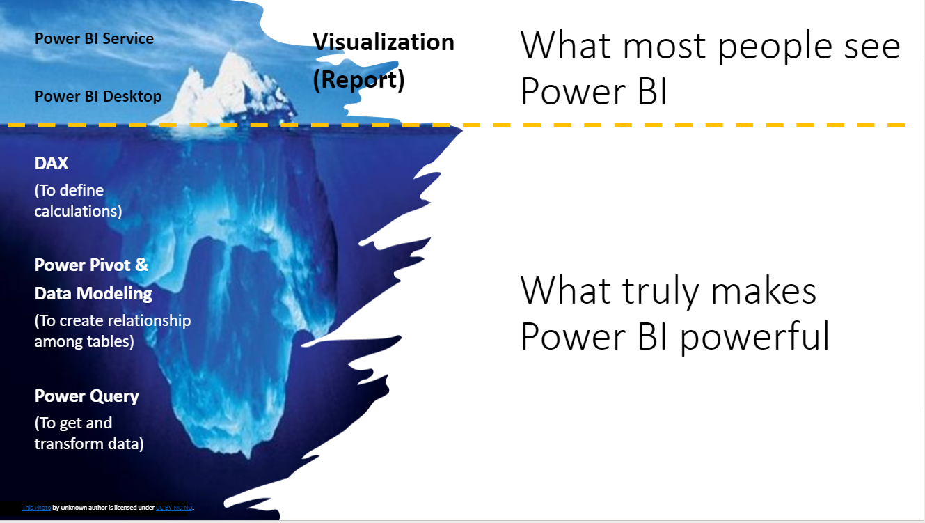
Power BI is a “relatively” new tool for analytics in business world. With no doubt, Power BI is getting more attention for its great power in visualizing data; in creating stunning dashboard; in getting insights from data by interacting with it, just to name a few. Many people think that Power BI is a visualization tool because this is what they “see” from a user’s perspective. This is super normal. However, what they don’t see, and probably are not aware of, are the building blocks behind the sense.
Hey, don’t get me wrong. These are not the building blocks I talked about.
These are the building blocks of reports/dashboard though
From my experience, these are the starting points most users user/learn Power BI. It happened because they are users of Power BI report that is created by IT (or someone else). They don’t need to worry about (indeed have no idea) how the data is being pull together from various data sources (where Power Query plays a crucial role); they don’t need to worry anything about Data Model or Power Pivot (how different tables are linked together through relationship); and they have never heard of DAX because they don’t have to. Without any knowledge just mentioned, they are still able to use the report to get information they need.
Regardless of what we do with Excel, Copy and Paste is something we do on daily basis… or even hourly basis. 😁
You may be thinking, every one knows Copy and Paste. Yes, probably. But is every one using Copy and Paste efficiently? In this short video, I will show you 7 Copy and Paste tricks that I wish I knew sooner. Check it out!
Think about this… you have spent hours of work building your wonderful Excel template. Needless to say there are lots of formulas that took you hours of thorough thoughts and considerations, on top of the beautiful formats and layouts. You are very happy with it and you share it to your colleagues. Just a few minutes later, your colleague came to you and said your formula did not work; many errors came out; and seems that someone had “carelessly” messed up some formats and layouts…
You opened the workbook and you found that someone
deleted rows and columns that they are not suppose to…
inserted rows and columns at wrong positions…
applied different color-filled and font sizes in an ugly way…
and many more…
Your mood travelled from heaven to hell in just a few minutes.
Is it familiar to you? If it is, you have to know how to protect yourself cells from editing.
It is super easy to move cells around by drag and drop. The standard drag and drop action however replaces contents in the destination cells. What if we want to preserve destination cells and just shift them up or right? A simple mouse trick could help.
Disclosure: The author earns a small amount of commission (at no additional cost to you) for the product/service successfully sold through the links of [Affiliate].
Wanna buy me a drink!?
Click below photo to my PayPal.Me
I appreciate it. :)