There are many ways to find out the cells in column B which are different from the cells in column A, e.g. using Conditional Formatting, Using formula in column C. These methods require some knowledge in Formula. Nevertheless, It could be a headache to many people with “formula-phobia”… ;p
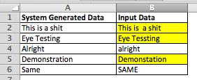
Look at the screenshot below. The task is to highlight the cells in column B that are different from that in column A. OMG, is it an eye-test?

No worry. A few clicks can accomplish it.
1) Select the range for comparison. A2:B6 in this example
2) “Ctrl G” to open the Go to dialogue box –> Special –> Row Differences

3) Bingo! Now simply apply the format you like to highlight the cells selected.

4) Here you go!
Note:
- As you see, the result is not case-sensitive
- If you select more than 2 columns, comparison will be made to cells in the leftmost column.
- If you understand Row Differences, you probably understand Column Differences which serves the same purpose in different orientation.
A simple spreadsheet you can manage is better than a sophisticated spreadsheet you need help.


