Happy New Year! Wish you all an Excellent Year of 2022!

To kickstart the year, let’s share a trick to solve a common task – highlighting differences in two ranges, with conditional formatting.

Common enough, right?

The ingredients are simple, for most cases, what we need to know are

1. The formula to compare two cells, e.g. =A1=F1 (in this example);
2. The location to put this formula for Conditional Formatting

Are you ready? You may download a sample file to follow along:

Let’s watch it in action:

If you prefer reading to watching, please continue…

1. Select the range you’d like to highlight where differences are (note: the range selected should be of the same size as the comparison range)
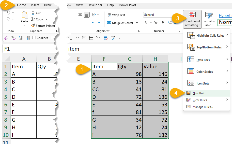
2. Go to Home tab
3. Select Conditional Formatting
4. Select New Rule…

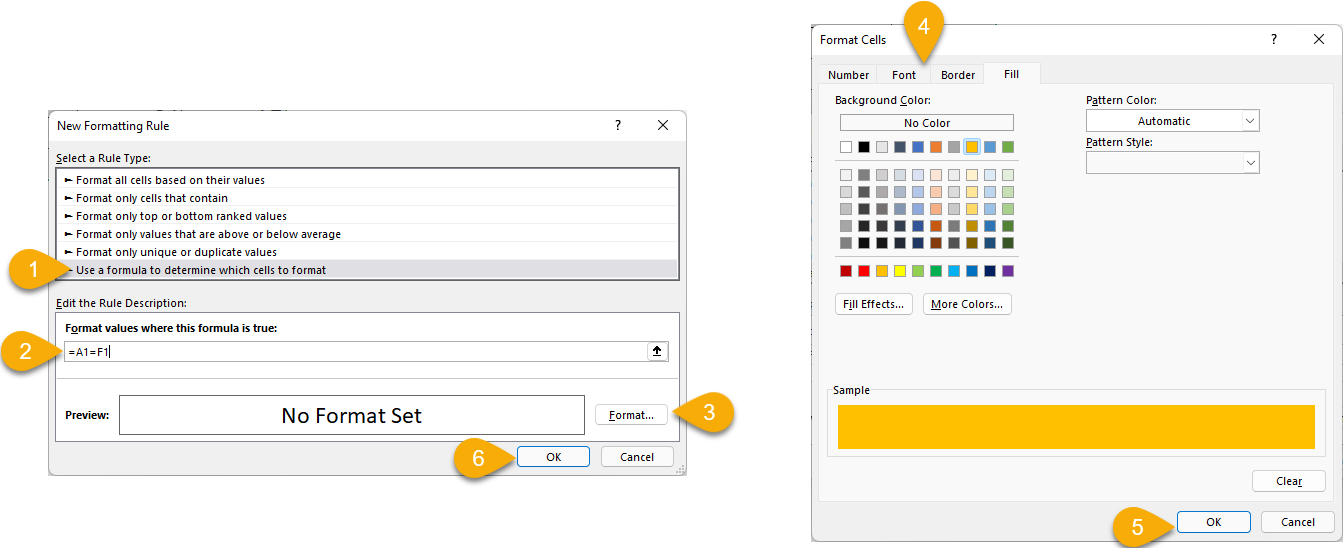
In the subsequent dialogue box,

1. Select “Use a formula to determine which cells to format (isn’t it self-explanatory?)
2. Type “=A1<>F1” (without double quotation marks)
3. Format…
4. Pick the format(s) you like (in this example, light yellow filled)
5. OK
6. OK again

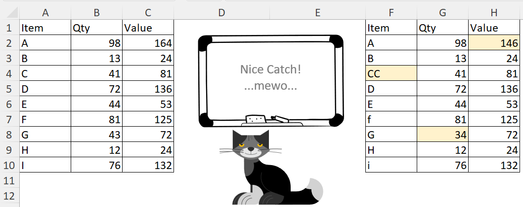
As simple as this! 😉

Although it seems to be easy, many people failed to do it at first attempt. The main reason for the failure is the use of $.

Please pay attention to the formula we used:

= A1 <> F1

Here’s the fundamental importance:

1. Both A1 and F1 are relative references (both column and row), i.e. no $ sign used
2. Both A1 and F1 are the upper leftmost cell in the two ranges
3. And the “Applied to” ($F$1:$H$10, this range is both column and row absolute), which is where we selected before clicking the Conditional Formatting button,

In plain English, these rules ask Excel to look into the range of F1:H10, compare the corresponding cell value in the range starting from A1, cell by cell, then highlight the differences (this is where the formula =A1<>F1 plays the role).

It would be easier to “visualize” it indeed:

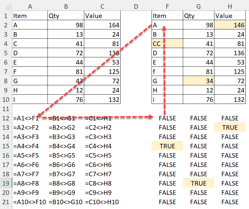
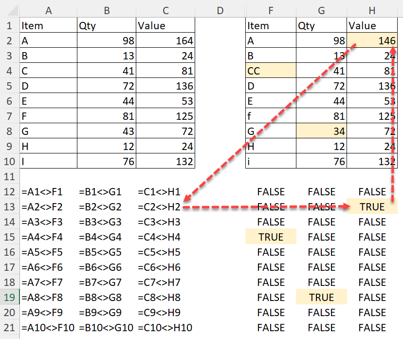
Imagine this, for the range F1:H10 there are invisible formulas behind the scenes to determine if a cell should be formatted or not. And the invisible formula is

= A1 <> F1

Since both A1 and F1 are relative, it moves across and down with the active cell. Basically,

In F1, it checks if A1 <> F1, which is FALSE ==> not formatted

In G1, it checks if B1 <> G1, which is FALSE ==> not formatted

In H1, it checks if C1 <> H1, which is FALSE ==> not formatted

…

In H2, it checks if C2<>H2, which is TRUE ==> formatted

……

Until it checks the last cell in the range, i.e.

In H10, whether C10 <> H10, which is FALSE ==> not formatted

When you get this clear, using formula in conditional formatting is secret no more. We just need to pay attention to where we put the $. 🙂

At this point, you may notice that the formula we used in the above example is case insensitive. It fails to differentiate “f” from “F”. In case we want to do it in a case sensitive way, the following formula would do:

= NOT(EXACT(A1,F1))

EXACT takes two arguments. It compares if the two inputs are exactly the same. Nevertheless, we want to highlight differences rather than same, thus we wrapped it with NOT. In short, it instructs Excel to format those are not exactly the same.

Did you catch a typo? Please leave your comments. 🎉🐱