Totally forgot I put my first post here 5 years ago. Time really flies! Thanks for flying with me. 🙂

Totally forgot I put my first post here 5 years ago. Time really flies! Thanks for flying with me. 🙂
Last week, I told you that my Surface Pro 4 is out of service, and I am waiting for a new laptop for writing my Excel blog… until late September or early October. That was the plan.
Although I am having a “late” summer break for writing excel tips and tricks for now, nothing stops me from learning new Excel stuffs. This morning, I watched MrExcel.com’s YouTube channel and heard MrExcel (Bill Jelen) said: “If you have a channel and you have viewers and you can reach people, please pass this note along“…
That was the moment. Yeah… Why don’t I share something cool! Even though I am not using Excel 365, it’s good to know what’s new and keep updated.
Here’s the MrExcel’s video talking about one of the cool features of Excel 365 – Threaded Comments:
Hope you enjoy it. 🙂
Today, I am not talking about Excel although I would like to. Why? Because my Surface Pro 4 is out of service… 😦
It has been out of order a few weeks ago… the moment when the warranty period was just expired. I was struggling whether I should fix it, or I should buy a new one. To fix a Surface Pro is not an easy task to my understanding. Worst still, there is no official repairing service in Hong Kong. When I contacted Microsoft, they offered to replace my Surface Pro 4 at a cost, which is actually not cheap given the fact that they are not going to replace me with a new machine….. @_@
On top of my mind is to buy a New Surface Pro. Indeed, I like the usage experience of my Surface Pro 4 very much. It’s an excellent replacement of traditional notebook: Light in weight with high performance (good enough for writing Excel blog). Also, I like the touch screen and Surface Pen with that I can write on captured screens (to have sort of a personal touch to my illustration, although I know that my handwriting is poor. :P) However, I am afraid that it will be broken in 13 months… even though I know it’s just a random event totally depends on luck. A friend told me that I should buy the extended warranty. For a machine that does not break down in three years, it probably can last for long. He’s got his point, I believe. But one of my considerations, after my Surface Pro 4 broke-down, is “Fixability”. I prefer something that is fixable and can last for long as I don’t want to throw away a machine simply because one of the components went wrong.
Another consideration is not about the performance of the machine, but my commitment to this blog. You know what… I felt a bit “emptiness” for not writing anything about Excel in the past few weeks. I know that I am abnormal, sort of. ;p Therefore I am looking into other options such as traditional notebook, which is in most cases more repairing friendly.
After browsing and browsing, windows shopping and windows shopping, I have decided to buy a new notebook, which will be arriving in mid September. Coincidently, I will be traveling for leisure for two weeks in mid September. That means, I won’t be able to start writing about Excel until end of September, or early October. Let’s consider it a belated summer break for myself.
Meanwhile, I will take the time to plan for the topics afterwards. Stay tuned, Stay Excellent. 🙂
 Photo by me. 🙂
Did I tell you that besides Excel, I enjoy hiking and taking photos.

Feel free to share this formula to your friend / colleague whom you think applicable… 🙂

He/She knows the answer. 😛

In retail, it’s very common to compare sales of same day, not same date, of last year. If you are not in retail sector, you may wonder what is the difference between same day and same date of last year.
Let’s look at example:
Assume today is 2018/08/11, and same date of last year is 2017/08/11. Very straight forward.
But retail people will never compare YoY sales performance in this way. Why? Because it compares apple to orange. Think about this, sales on Saturday (2018/08/11) should be better than Friday (2017/08/11). Make sense? So we want to compare 2018/08/11 to 2017/08/12 instead. It’s a Saturday to Saturday comparison.
As such, there is constant demand for Excel formula to get the same day of last year. In many cases, Excel user would use functions related to date. Continue reading

To load an Excel Table into Power Query is easy. Just click into any cell of the Excel Table, and then click the From Table/Range button (depends on which version you are using, this button resides in different location on the ribbon). This action will take your active Excel Table to the Power Query Editor. To load another Excel table, we need to close the Power Query Editor, go to the Table, then repeat the step. Easy, Piece of cake.
However, when you have 20 Excel Tables and you want to load all of them into Power Query, you need to repeat the steps 20 times. Not really a nice experience. 😦
To my limited knowledge to Power Query, there is no simple way to load multiple Excel Tables as separate queries in one step. Please correct me if I am wrong. ;p I tried to Google it, but no success.
Nevertheless, there could be a “quicker” way to do so, just a bit quicker… Continue reading
This is a short story of mine, and an imaginary conversation in my head…
This was a question from a colleague sitting opposite to me. My quick response was: “Yes… but it is a bit, just a bit complicated…”As I was doing something else, I didn’t answer him right away. Then after a while, he told me he “googled” the formula he needed. That’s fine.When I finished my task, I asked him for the formula he’s got… then I provided him my formula (a shorter one). :PThat’s the end of the story, but the beginning of my thought:
Is it good to have an Excel “nerd” sitting around you?
Most people would say YES, I guess, because they can have quick answer to their Excel questions.However, I think the opposite. It may indeed slow down your learning curve in Excel.Indeed what I meant “complicated” in the beginning is that it requires nested functions. The solution is not complicated. We just need to know three functions:
Looking back, if I was not occupied by other tasks, I would continue our conversation like the following: Continue reading
This post is about showing you how to perform a common task of adding a column of
with Quick Analysis in Excel 2013 or later.
Well, what I meant “latest Excel” here are those versions since Excel 2013. Of course, Excel 2016 and of course Excel 365 is getting even better.
You may think that Excel 2013 is a product of 5 years ago… there is no way it can be called “latest”…. uuuum… that’s true. However I am living in a city where most people I know (across different companies) are still using Excel 2010 or before. Believe it or not? 😛
What is even more surprising (or ironic): when I met someone who uses Excel 2013 or later, I looked at them with my “hearty” smiles and told them how lucky they are with all those new features like Flash Fill, Quick Analysis, etc….. (not yet to mention about the new FUNCTIONS). The response I got was mostly: “What are these?” and some of them unconsciously showed an attitude of “I don’t care…”
Needless to say, many people have never clicked the tiny icon that showed up automatically when a range of data is selected.
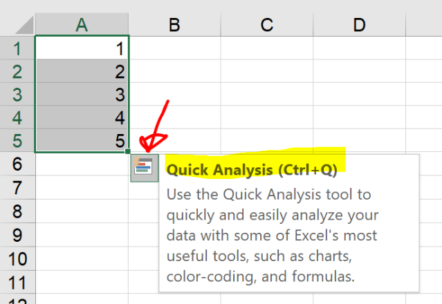
So, I am going to show one quick tip of using Quick Analysis (provided that you are using Excel 2013 or later) to add a column of
A picture (especially an animated one) tells thousand words, so let’s look at the screencast below: Continue reading
With no doubt, combining multiple tables (mostly on different worksheets, or even in different files) into a single “master” table for further analyses is one of the most tedious tasks we deal with Excel day to day. Inevitably, manual Copy and Paste is the go-to option (unless you are VBA expert). Sometimes, the tables we are trying to combine contain different columns. You know that feeling of frustration, don’t you?
With Power Query, we can say NO MORE to copy and paste for this tedious task. In this post, I am going to show you what Append Query does, and some interesting notes of it.
I will demonstrate how Power Query appends tables for four different cases: Continue reading
![]()
Recently I am quite busy (and moody) at work, I mean the real work at office. You must be thinking my works involved using Excel a lot and I should be able to finish them in an efficient way. However the fact is… Excel is the barely opened application in my PC at work. When I use Excel at work, I probably use it for “non-analytic” purposes. Can’t imagine, right?
Then one day, I received an email from Feedspot saying that wmfexcel.com has been selected as one of the Top 40 Excel Blogs. That was the truly refreshing moment of my boring day.
Frankly speaking, I think I have not reached this level yet. Nevertheless I am super happy that my blog is getting more popularity. If you are reading this, I sincerely thank you! 🙂
Do you use VLOOKUP? If you do, you should know there are limitations to VLOOKUP. Also, there are some cases VLOOKUP is not straightforward and efficient.
Consider the following cases: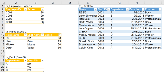
What we want to achieve is to map the corresponding staff information (in the lookup table, named tb_StaffInfo) to the orange tables (named as tb_Employee, tb_Name, tb_Dept) on the left.
Case 1: Although there is a common key (EmployeeID vs. Staff ID) in both tables, the lookup direction for Name is to the left which an ordinary VLOOKUP fails to accomplish. Read here to learn more about this limitation and an alternative way to overcome this.
Case 2: There is no common key, we may need to combine First Name and Last Name in tb_Name first to get the common key, or to split the Full Name in the lookup table into First and Last Names, then do VLOOKUP 2 values. Either way, it’s not direct.
Case 3: Duplicate record (Dept) in the lookup table. We know that VLOOKUP will only return the first match in the lookup table. VLOOKUP cannot return all the matching records in the lookup table.
Power Query, however, overcomes these challenges with ease.
You may download a Sample FIle – Doing complicated vlookup with PQ (Start) to follow along.
Sometimes we want to add a descriptive like “Good Job” for figures above target; “Work Harder” for those below… like the following screenshot:
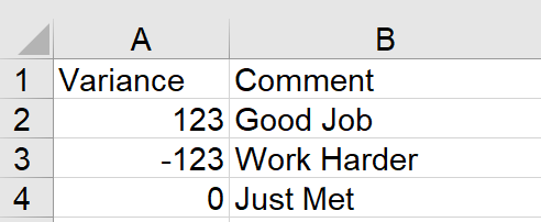
To many people, the top-of-mind solution should be using IF function.
=IF(A2>0, "Good Job", IF(A2=0, "Just Met","Work Harder"))
This formula does the job fairly easy! 🙂
One drawback is, we will need a helper column to achieve this. In some cases, we want the descriptives only; showing the numbers is not necessary. For this case, Custom Format should be the go-to approach.
Format Cells –> Number Tab –> Custom –> Input the following into Type: Continue reading
This is my first post devoting to my recent love for Excel – Power Query. 🙂
First, let me make myself clear. I am still learning Power Query (indeed I am still learning Excel too). The more I learn and use Power Query, the more Excel power I get. Frankly, I am far away from being an expert in Power Query. Having said that, I am “relatively” good by knowing how to use many Magical commands through the super-friendly User Interface of Power Query. Together with a little knowledge in editing auto-generated codes in formula bar of Query Editor, I feel like I can fly with Excel. 🙂
In this post, I am trying to show you how to solve a workplace problem, that is quite complicated if using Excel alone.
Warning: This is a long post.
We all know that shortcuts could save us lots of time when working with Excel. Excel has many built-in shortcuts. Ctrl+C, Ctrl+V should be the most popular and commonly used ones as most of us are doing copy and paste daily, or even hourly. ;p Just to name a few more, Ctrl+1 to format cells, Ctrl+S to Save, Ctrl+F to Find are some other commonly used shortcuts using Ctrl+ Key combinations.
However, there are some actions you would not find the Ctrl+ shortcut for it, e.g. Format Painter, Sort A to Z, Align (selected objects) Top, etc…
But did you know that we can access to almost all buttons on Ribbon and QAT by using Alt key combinations?
In this post, I am going to show you how to find out the Alt keys combination for actions you find on Ribbon, and more importantly, how to put your favorite (most frequently used) actions onto QAT for enhanced productivity.
I am having an incentive trip in Osaka… not sure if this is due to my Excel skills. 😛
So let’s have fun this week. 🙂

What would you say if you were the interviewer? Leave it in comments. 🙂
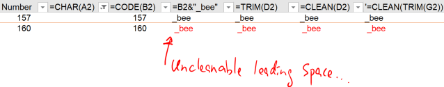
To fix this problem, we need to understand where is the “leading space” coming come. Before we jump to that, I want to show you two Excel functions first:
CHAR returns the character specified by a number. Use CHAR to translate code page numbers you might get from files on other types of computers into characters. (Source: Office Support )
CODE returns a numeric code for the first character in a text string. The returned code corresponds to the character set used by your computer. (Source: Office Support)
| Operating environment | Character set |
| Macintosh | Macintosh character set |
| Windows | ANSI |

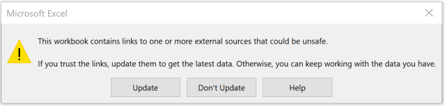
When we have created a wonderful #Excel template that is to be shared with others, we don’t want users to distort, if not destroy, the template someday. Nevertheless we would like to leave as much “flexibility” as possible to users by not password-protecting anything on the template. We know that some users are super creative to crack a password-protected sheet/book. 😛
It is simple to make a READ ONLY file. Continue reading
![]()


New Generation Finance - Accounting - Controlling using Microsoft BI stack
A Power BI Creator Blog
Work smarter by Mastering Functions in Excel
Work smarter by Mastering Functions in Excel
Helping lawyers make the most of Microsoft Excel
Work smarter by Mastering Functions in Excel
Work smarter by Mastering Functions in Excel
Work smarter by Mastering Functions in Excel
Peltier Technical Services - Excel Charts and Programming
Turn your data into opportunities
Q&A about Excel
Doug Glancy's Excel Site