Do you use VLOOKUP?  If you do, you should know there are limitations to VLOOKUP.  Also, there are some cases VLOOKUP is not straightforward and efficient.

Consider the following cases: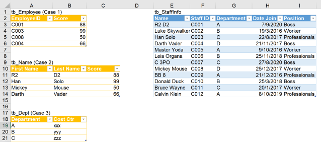

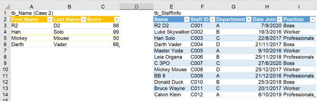
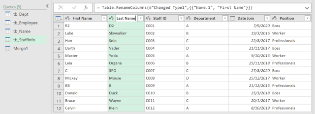
What we want to achieve is to map the corresponding staff information (in the lookup table, named tb_StaffInfo) to the orange tables (named as tb_Employee, tb_Name, tb_Dept) on the left.

The challenge

Case 1: Although there is a common key (EmployeeID vs. Staff ID) in both tables, the lookup direction for Name is to the left which an ordinary VLOOKUP fails to accomplish. Read here to learn more about this limitation and an alternative way to overcome this.

Case 2: There is no common key, we may need to combine First Name and Last Name in tb_Name first to get the common key, or to split the Full Name in the lookup table into First and Last Names, then do VLOOKUP 2 values.  Either way, it’s not direct.

Case 3: Duplicate record (Dept) in the lookup table.  We know that VLOOKUP will only return the first match in the lookup table.  VLOOKUP cannot return all the matching records in the lookup table.

Power Query, however, overcomes these challenges with ease.

You may download a Sample FIle – Doing complicated vlookup with PQ (Start) to follow along.

Note: All screenshots are prepared using Excel 365, which Power Query is renamed as Get and Transform, under the Data tab.  If you are using Power Query for Excel 2010 or 2013, you may find the icons at different locations on your Ribbon, where Power Query has its own tab.  Nevertheless, the flow should be more or less the same.

Let’s VLOOKUP the Power Query way

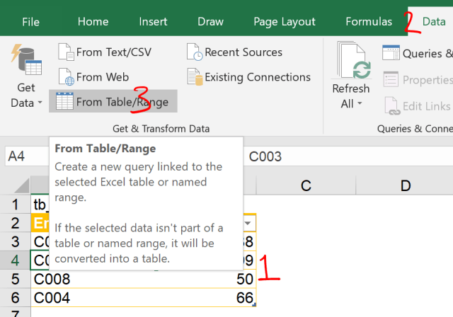
First of all,  load all tables into Power Query

1.  Select any name in the Table
2. Go to Data –> Get & Transform Data
3. From Table/Range

Tip: We may need to edit the “Changed Type” here.  Since our dataset is quite simple here, Power Query detects the data type of each column correctly.

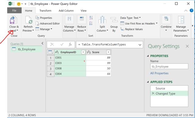
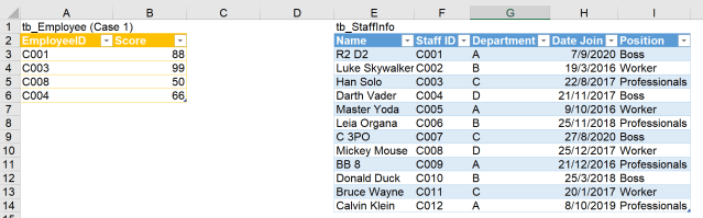
Now Close & Load To…  Only Create Connection

Repeat the above steps to load the other three tables.

Now we are ready to VLOOKUP the Power Query way.

Case 1 – VLOOKUP to the left

Challenge: The common key is “EmployeeID” and “StaffID”, but we also want the information “Name” which is on the left-hand side of the key.

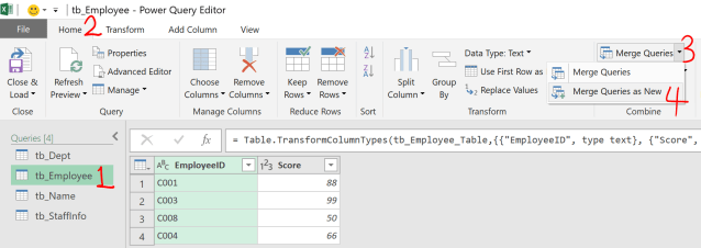
Let’s go to the Power Query Editor by double-clicking one of the queries in the Queries & Connections pane:

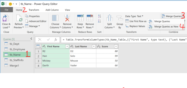
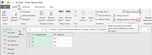
Merge Queries

1. Select the base query, i.e. tb_Employee” we need
2. Go to Home Tab
3. Merge Queries…
4. … as New

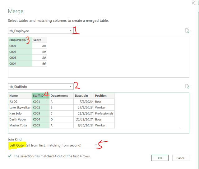
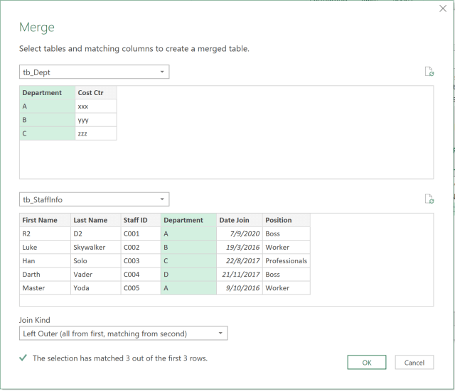
Now the Merge table dialog box opens:

1. Select the base table tb_Employee
2. Select the lookup table tb_StaffInfo
3. Select the common key in base table “EmployeeID”
4. Select the common key in lookup table “StaffID”
5. Select Left Outer Join Kind

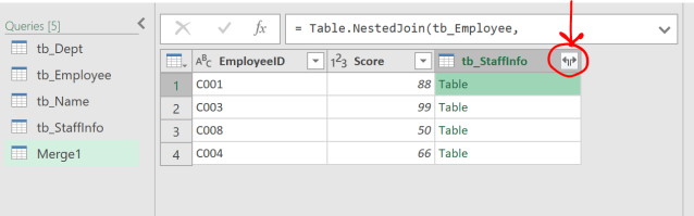
Once we hit OK, we will see the merged query called Merge1 as follow:

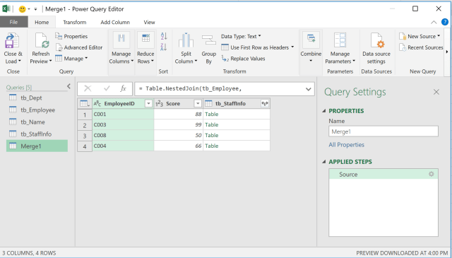
Very different from traditional VLOOKUP, we won’t see any lookup values at this point. Instead, we see a column called “tb_StaffInfo”, which is basically the name of the query just merged.  And under this column, there is only “Table”… nothing else.

Let’s click into the cell of “Table” and observe (the lower pane):

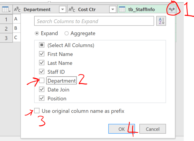
The “Table” contains all the columns of the matching record (EmployeeID).  What we need is to click the “Double open arrows” icon on the header to get expand the columns:

• Uncheck “Staff ID” as it is essentially the same as the “EmployeeID”.
• Also uncheck “Use original column name as prefix”

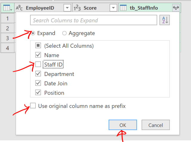
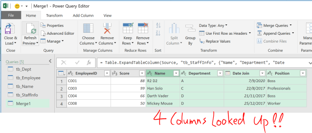
Hit OK.  Wahlala…… 4 columns, of which 1 column “Name” was on the left to the common key, were looked up correctly!

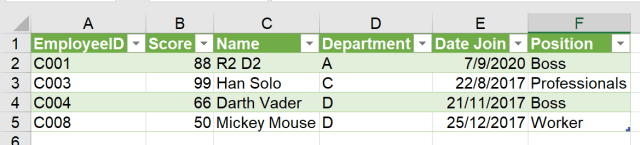
Now, load it to A1 of Result(1) as Table:

==>  

Case 1 solved!  Isn’t it easy?

Case 2 – VLOOKUP 2 values

Challenge: There is no single common key.  We need to lookup 2 matching values.

To do this, we may either

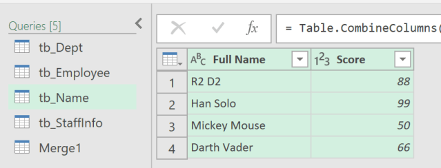
1. In the tb_Name query, combine First Name and Last Name into Full Name, so that we have one common key:

or

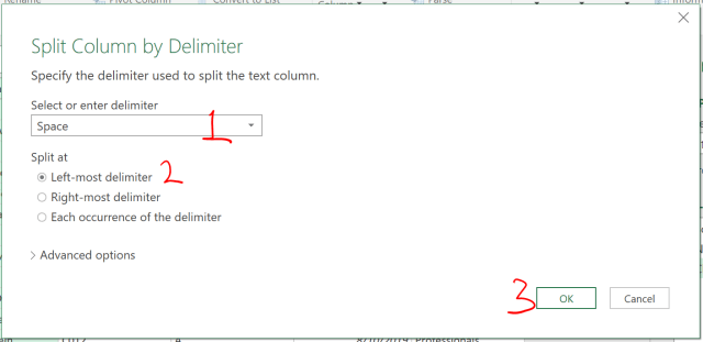
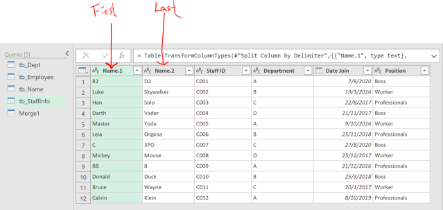
2. Split the Name column in the query tb_StaffInfo into First Name and Last Name, so that we have two common keys to do the mapping:

Double click the header to rename it:

For the 1st method, the Merge Queries step is the same as shown in Case 1.  No need to repeat here.

Let’s see how to Merge Queries based on two lookup values, i.e. First Name and Last Name in this example:

Merge Queries as New

When the Merge Queries dialog box is opened:

1. Select the base query tb_Name
2. Select the lookup query tb_StaffInfo
3. Click First Name under tb_Name
4. Click Last Name under tb_Name
5. Click First Name under tb_StaffInfo
6. Click Last Name under tb_StaffIno
7. Select Left Outer Join Kind

Note: the sequence in steps 3-6 are crucial.  You will see the tiny number next to the headers that shows you the sequence of selection.

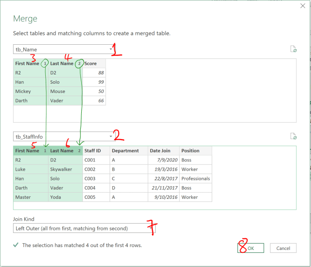
8. Hit OK

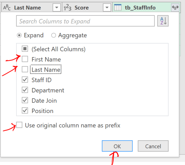
Now the queries are merged as Merge2.  Click the “Double open arrows” icon to expand the columns needed:

Uncheck fields that we don’t want.  Put it in other words, select fields we need:

Load the result to a A1 of Result(2) as Table:

Here we go!  Case 2 solved.

Information is mapped based on 2 values: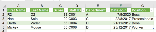

Case 3 – Get all matching records from lookup table

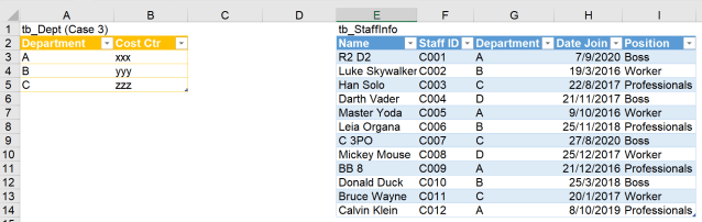
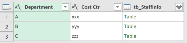
Challenge: We want to get all information for Department A, B, C that is listed in tb_Dept, from the lookup table tb_StaffInfo.

There are 4, 3, and 3 records of Department A, B, and C respectively.  VLOOKUP cannot do it.  No way it can… 😦

Imagine how we do it with regular Excel (assuming no VBA).  We would probably need Advanced Filter to get all matching records from tb_StaffInfo, then map the “Cost Ctr” back to the filtered result… Quite tedious, not to mention our data is so simple here for demonstration purposes.  What if we have 10 columns in tb_Dept… Can’t imagine.  😦

Let Power Query do the Magic

If you have been following along, you should know the steps of Merging Queries well.  So just repeat the Merge Queries steps to merge the query tb_Dept with tb_StaffInfo:

Up to this point, let’s see what do we have for each “Table” in the Merge3 query.

Do you see the difference?  Before, when there are no duplicates on the matching key in the lookup table, there was only one row returned for each table.  Now for Department A which we have four records in the lookup table, the merged Table contains all four records.  Same for Department B and C, where the Table contains 3 and 3 records respectively.

Let’s click the magical “Double open arrows” to expand the fields we need:

Three rows of data turn into 10 rows, showing all records for Department A to C.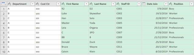

Let’s sort the column Department to make it good looking: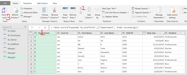

Now, let’s load it to A1 of Result(3) as Table:

Here we go!  Case 3 solved with ease!

Don’t forget, what makes Power Query so amazing is its ability to do the whole transformation with a single click of Refresh when new data comes.  See below screencast in action:

Simply awesome.  🙂

Do you feel the Power?

You may download the Sample FIle – Doing complicated vlookup with PQ (Finished) with the queries to view the steps.