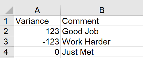
Sometimes we want to add a descriptive like “Good Job” for figures above target; “Work Harder” for those below… like the following screenshot:

To many people, the top-of-mind solution should be using IF function.

=IF(A2>0, "Good Job", IF(A2=0, "Just Met","Work Harder"))

This formula does the job fairly easy! 🙂

One drawback is, we will need a helper column to achieve this.  In some cases, we want the descriptives only; showing the numbers is not necessary.  For this case, Custom Format should be the go-to approach.

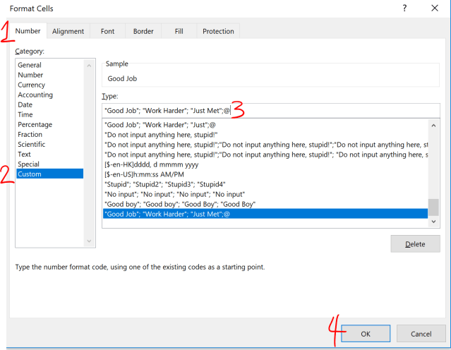
Format Cells –> Number Tab –> Custom –> Input the following into Type:  

Here’s the result:

See the values in formula bar vs. the cell contents?!

That is the result from the following custom format:

"Good Job"; "Work Harder"; "Just Met";@

The custom format comes with four portions: Positive Number; Negative Number; Zero; Text (separate by ; ) 

So the above custom format means:

• For positive number –> Display “Good Job”
• For negative number –> Display “Work Harder”
• For zero –> Display “Just Met”
• For text –> Display whatever input (as represent by the @ symbol)

Note: We need double quote “” for text to be displayed

As simple as this.

You may download a Sample File to follow along.

Want some fun with your colleague?

"Silly"; "Silly"; "Silly"; "Silly"

No matter what the user input into cells with this custom format, s/he will only see the word “Silly”.

OR

You may put secret messages to someone whom you wish to express your special feelings to:

"Love you"; "Think of you"; "Miss you"; "???? You"

Disclaimer: Do it at your own risk. 😛

For more about custom format, you may refer to this page from support.office.