Feel the Power (Query)

This is my first post devoting to my recent love for Excel – Power Query.  🙂

First, let me make myself clear.  I am still learning Power Query (indeed I am still learning Excel too).  The more I learn and use Power Query, the more Excel power I get.  Frankly, I am far away from being an expert in Power Query.  Having said that, I am “relatively” good by knowing how to use many Magical commands through the super-friendly User Interface of Power Query.  Together with a little knowledge in editing auto-generated codes in formula bar of Query Editor, I feel like I can fly with Excel.  🙂

In this post, I am trying to show you how to solve a workplace problem, that is quite complicated if using Excel alone.

Warning: This is a long post.

The routine task

Imagine you need to maintain 8 price books (for 8 different markets) with more than 10,000 SKUs each.   From time to time, price of certain SKUs changes.  When it happens, you need to send the list of SKUs with new prices and effective dates to individual markets so as to provide them the information required for loading to local POS system.

To achieve that, you create 8 separate tables, listing all SKUs with coming price changes only.

The issue

As time goes by, there are so many tables with “new” prices; and “new” prices become “old” prices and obsolete.  Worst still, there is no Master Price Book showing the prices of each SKUs in different markets.

Because of this, you may need to go through each price book one by one in order to find the latest/coming price (or historical prices) of a particular SKU in a particular market.

My suggestion

When I heard about this (a real workplace case), I asked my colleague: “Why don’t you consolidate all data into a Master Price Book?”

She responded in doubt…… (skipping the details here. ;p)

…… I quickly drafted the data table below:

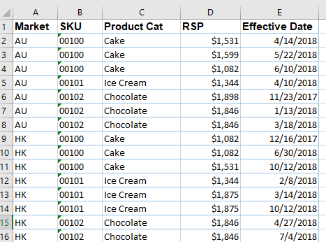
and said: “You may determine the Status of an item in a market based on the Effective Date, with the field “Status” you may get the information you need by Pivot Table easily”

A moment of silence…

Then she said something like… “It’s difficult and time consuming to update the status (manually)…”

Arrrrh…. I realized her concern which is so true:   She thought the “Status” needs to be maintained manually……

With Power Query, this is achievable with ease

Let’s not worry about how to combine the eight different files, as that is pretty easy with Power Query… ;p and this is not the topic of this post.

Our Objective

Based on the following dataset, assign three different status (“Current“, “Coming“, “Inactive“) to each row of the data.

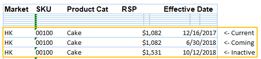
The logic is simple, when a record with effective date of a SKU in a market is:

• immediate future ==> its status is Coming
• immediate past or today ==> its status is Current
• Others ==> Inactive

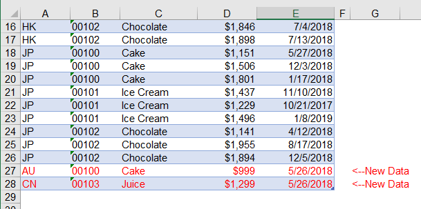
An example below (assume today is 5/26/2018):

Make sense?

If you are formula expert, you may be able to figure out an array formula to return the status of a SKU in a market based on the effective date.  However it is super complicated to write such an array formula to most of regular users.  And also think about the scale of data volume (>80,000 rows of record).  Array formula to return the status may not be an efficient approach.

Let’s do it the Power Query way

Note: All screenshots are prepared using Excel 365, which Power Query is renamed as Get and Transform, under the Data tab.  If you are using Power Query for Excel 2010 or 2013, you may find the icons at different locations on your Ribbon, where Power Query has its own tab.  Nevertheless, the flow should be more or less the same.

You may download a Sample File to follow along.

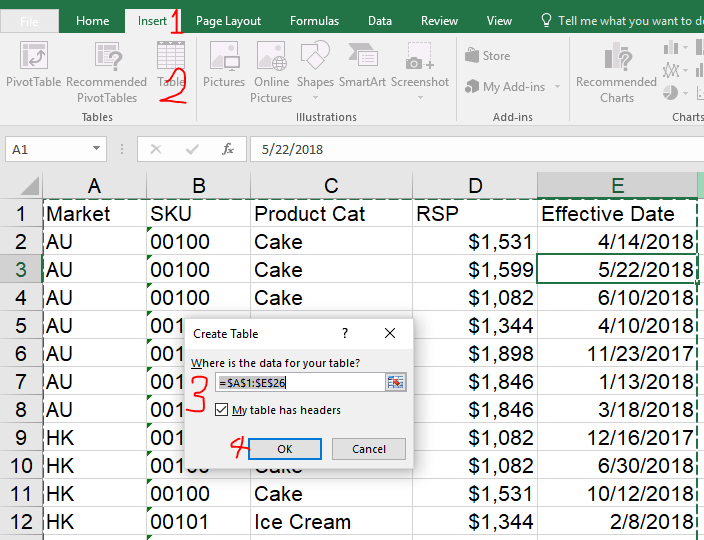
1. Turn the data range into Excel Table

1. Select the data range –> Go to Insert tab
2. Table  (Shortcut: Ctrl+T)
3. Confirm the data range; and tell Excel if “My table has headers”
4. OK

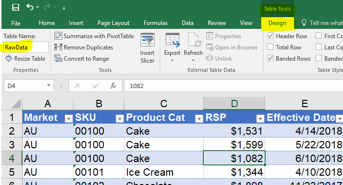
As a good practice, let’s give a more meaningful Table Name than “Table1”, e.g. RawData

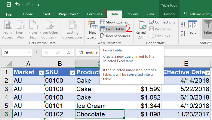
2. Load the Table to Power Query Editor

1. Select any cell of the Table you want to load to Power Query –> Go to Data Tab
2. From Table (Note: if your data range is not yet converted as Table, Excel will do it for you.)

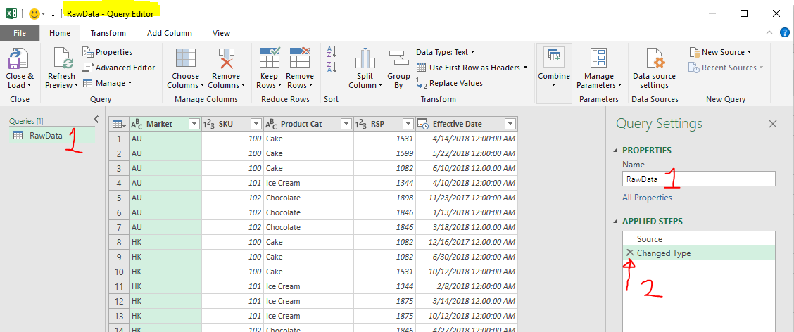
Now the table RawData is loaded to the Power Query Editor.  The following screenshot shows a preview of data (as our data set is small here, you see all rows of data in the preview).

Let’s rename the query to “BaseQuery”

1. Select the Query on the left pane –> Right-Click –> Rename or Change the Name directly from the right pane (Query Settings)
2. The step “Changed Type” is automatically generated; let’s delete this step by clicking the “x”  (Look at the preview data, did you see the data type for SKU changed to Number, which turns “00100” into “100” –> Something we don’t want…)

Let’s define the data type

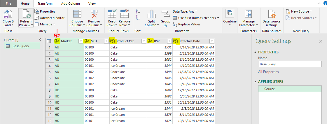
By clicking on the “ABC 123” icon on the left of column header, you will see a dropdown list of different data types for selection, which is quite intuitive: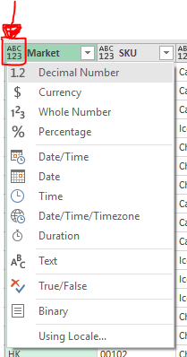 

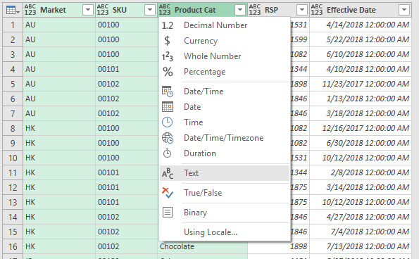
(Tip: We may apply the same data type to multiple columns by holding Ctrl key when selecting columns; remain holding the Ctrl key when clicking the “ABC 123” icon)

Let’s set the data type for each column as below:

1. Market / SKU / Product Cat as Text
2. RSP as Currency
3. Effective Date as Date

Now we have our BaseQuery set and ready.  We are going to reference this query for future steps.

3. Create a query for Current Price

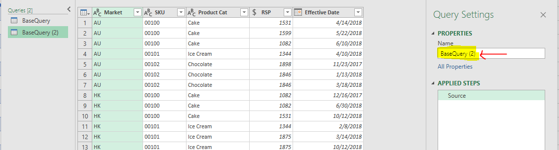
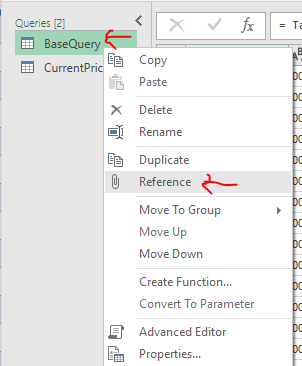
First, let’s reference the BaseQuery to create a new query:

Right-click the “BaseQuery” on the left pane –> Reference

Now we have “BaseQuery (2)” which is identical to the BaseQuery.  Let’s rename it to “CurrentPriceList”

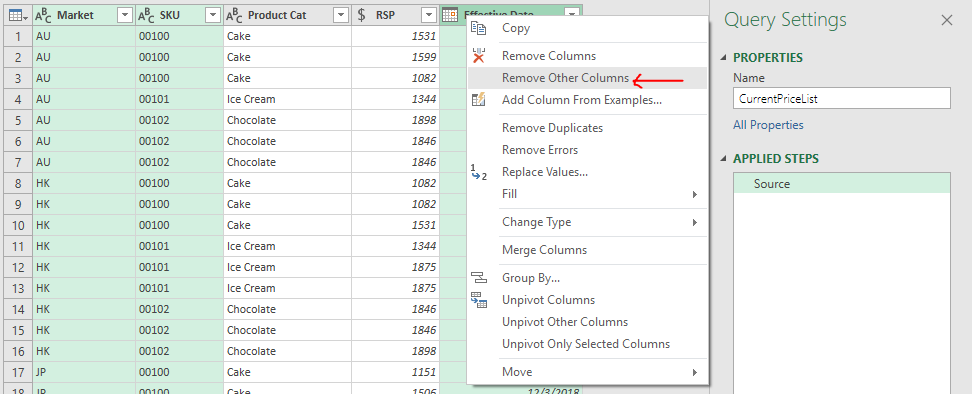
Keep only the columns we need

We will need three attributes (which are Market, SKU, and Effective Date) to define the price status of an item in a market, hence we can “Remove Other Columns”

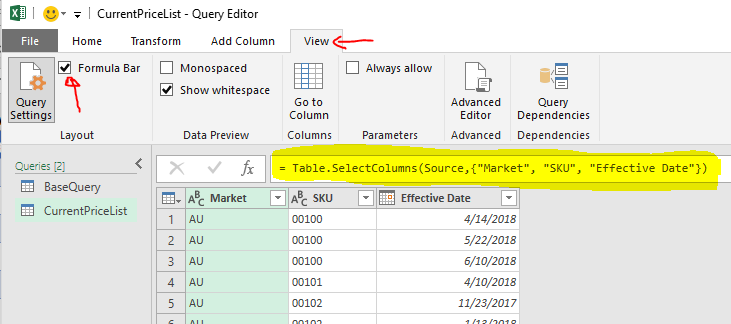
Let’s take a look at the formula bar.  For each action we did, Power Query generated a formula automatically.

Do you remember the logic of determining a price status?  For an item with more than one effective date, the one with the immediate past date (on / before today) is the Current price.  Make sense?

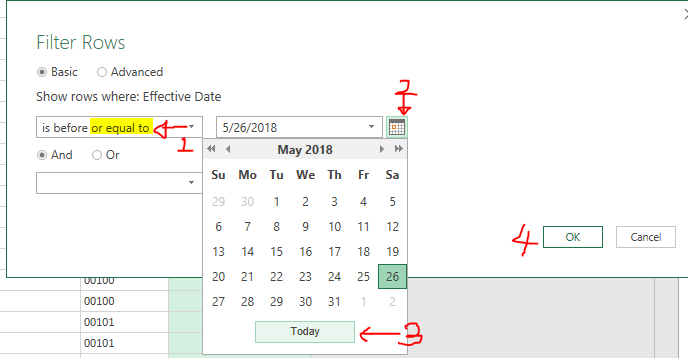
Let’s filter only effective dates on or before today:

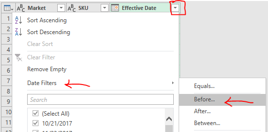
1. Select “is before or equal to”  (if the effective date is today, then its status is “Current”)
2. Click on the “Calendar” icon
3. Select “Today”
4. OK

Now, let’s have a look at the formula bar.

The filter is applied towards a “hard-code” date, which is 2018/5/26… No good.

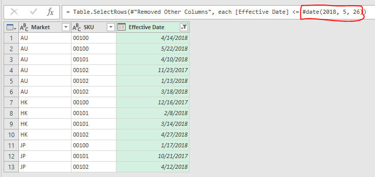
As an Excel guy, I tried to change that portion to “Today()”… but it did not work as the language behind Power Query is different.  There is no such Today function in Power Query.

The twist is to replace the #date(2018, 5, 26) with

Date.From(DateTime.LocalNow())

And it works perfectly. 🙂

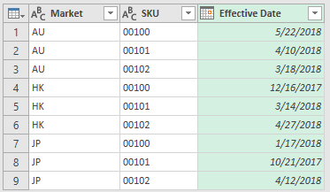
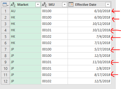
Now, examine the filtered data.  What we want is the list of items with “Current” status, which are highlighted below: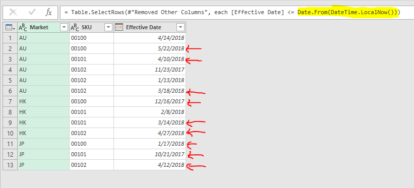

In natural language, we want to get the latest (biggest) Effective Date of a SKU in a market.

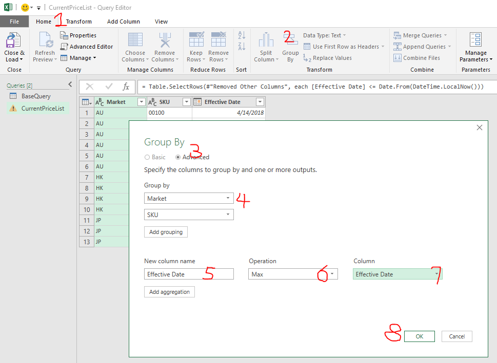
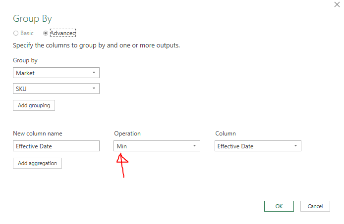
We can do it with Group By in Power Query:

1. Go to Home tab (of the ribbon on Query Editor, not the Excel)
2. Group by
3. Select “Advanced”
4. Group by Market, then Group by SKU (note: You may need to “Add grouping”)
5. Define a new column name –> Effective Date
6. Select Max under Operation (because we want to get the latest effective date)
7. Select “Effective Date” under Column, where we want the operation be applied to
8. OK

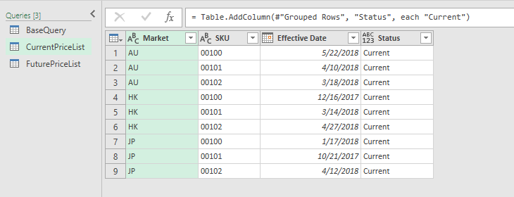
Here we go!  A list of SKU with the latest Effective Date that is on or before Today.

Let’s add a column to give them a proper marker.

1. Go to “Add Column” tab
2. Click Custom Column
3. Name the new column as “Status“
4. input = “Current”
5. OK

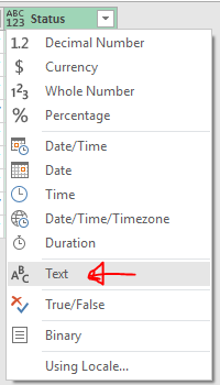
Don’t forget the change the data type to “Text” for the resulting new column just added.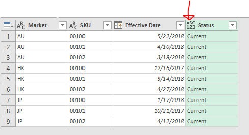

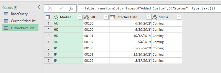
4. Create a query for Coming Price (i.e. the next future price)

First step is to “Reference” to the BaseQuery (again):

The steps afterward is 99% the same as the steps in Section 3.  So it’s better to illustrate through a screen-cast:

Did you time it?  It was done in less than 80 seconds.  🙂

Note the two major differences:

1. As we want to determine coming price, we filtered “>” Today instead of “<=“
2. To get the next effective date coming, we use “Min” for the operation in the steps for Group By.

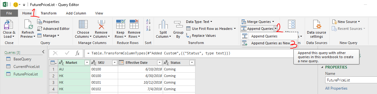
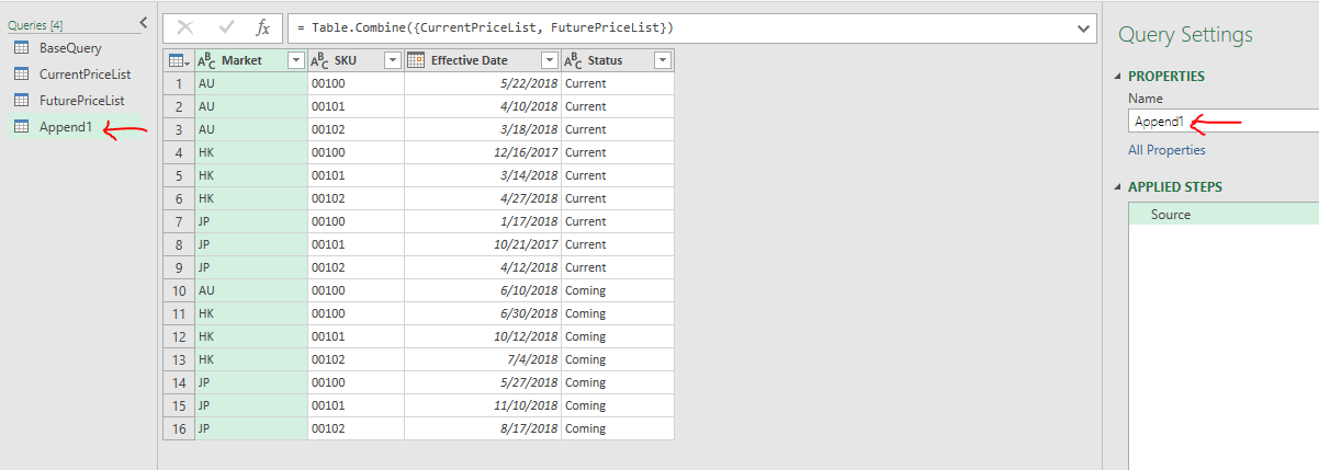
5. Append the two Queries

So far, we have created two queries: One contains list of items with Current status; one contains list of items with Coming status.

We want to feed this ” newly added” status to RawData.  Before we do so, let’s put the two queries into a single query :

1. Go to Home tab
2. Append Queries
3. Append Queries as New

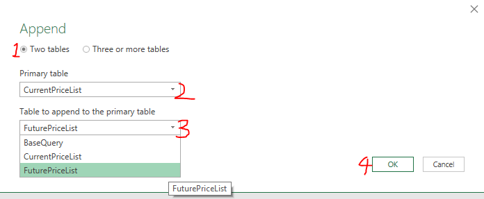
In our case, we have only Two tables to append.

1. Select “Two tables“
2. Select CurrentPriceList as Primary table
3. Select FuturePriceList as “Table to append to the primary table”
4. OK

Here we go!  An appended table showing list of items with status of both Current and Coming.

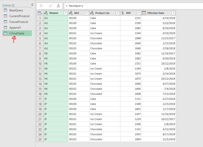
6. Feed the status back… by Merge Queries

First step is to “Reference” to the BaseQuery (again).

This time, I renamed it as f_FinalTable.  This will be the Table/Query we used for Pivot Table after all.

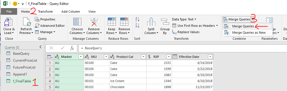
To Merge the queries

1. Select the f_FinalTable on the left pane
2. Go to Home tab
3. Merge Queries

• As we started with f_FinalTable, it is put on the top as “Left” table.
• Now select the Table (Append1) we want to merge with (consider this is a lookup table in Excel):
• Join Kind is set to “Left Outer” by default.  Leave it there as it is.

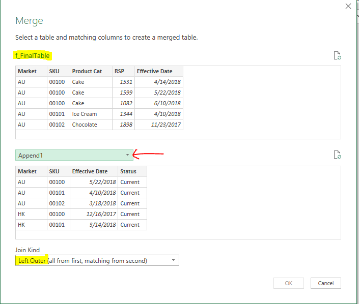
Now let’s select the matching columns on both tables.  Note, sequence does matter. Please be careful.  The following screen-cast demonstrates the flow (note: Hold Ctrl key when selecting columns):

When the matching columns are selected, we will see a summary at the bottom showing number of matched records.

Technically, it is a VLOOKUP with three lookup values.  You should know how tedious it is with regular Excel.

Now, we see a new column called “Append1”, the query name we just merged.

Let’s continue by clicking the “expand” icon:

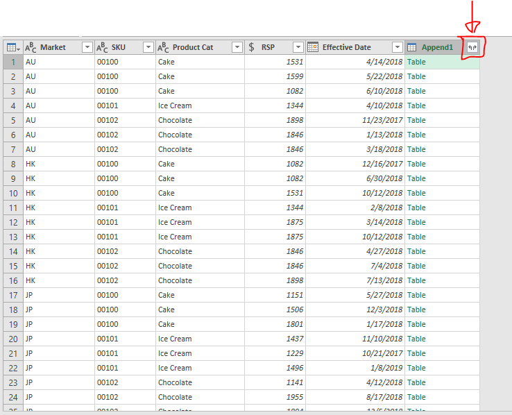
Check the field that we want.  In our case, “Status“.  Tip: Unckeck the “Use original column name as prefix”.

VLOOKUP with three values done successfully, with ease!

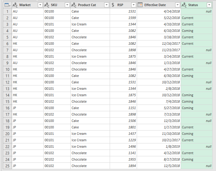
Wait… What “null” means?

For those non-matching records, null is returned.  What are the non-matching records? They are record of neither “Current” nor “Coming”.  In other words, they are “Inactive“.

arrrrrh.  That’s right.

Let’s replace “null” with “Inactive”.

1. Select the column “Status” in the f_FinalTable query
2. Go to Home tab
3. Replace Values
4. Value to Find: null, Replace with: Inactive
5. OK

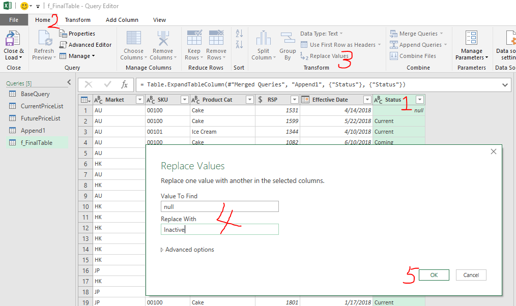
wakaka… it’s done in a flash. 🙂

To get a better view, let’s sort the result by 1) Market, 2) SKU, 3) Effective Date.  Then click Close & Load.

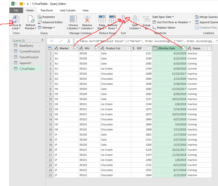
Result

Each query created is loaded to different worksheets.  And you will see a “Workbook Queries” pane on the right.  Click on a Query to go to the table loaded:

The true Power

If you have been following along, you may be thinking… well it takes quite many steps and they are not easy at all…  Is it worth doing so in this way?

Remember, we are dealing with a big table with more than 80k rows of record.  The table needs to be updated on regular basis.  Every time we update the price of certain SKUs (quite a lot indeed), we want to retrieve updated information easily (and quickly, means in minute not hour) to show list of current / coming price with effective date by market.  It’s not an easy task with regular Excel.

With Power Query, and the steps we created, this tedious task becomes a click of Refresh.

Here’s the sample file with the queries: Sample File – Maintain Price Book Using Power Query (Finished)   (Please Enable Content when prompted) 

Let’s see the Power in action.

Suppose we have new data added to RawData.

To get the updated information, simply go the the query loaded, right-click and Refresh.  As simple as this!

Isn’t it easy but powerful?

The following diagram illustrates the flow of the queries created.  Simply awesome!

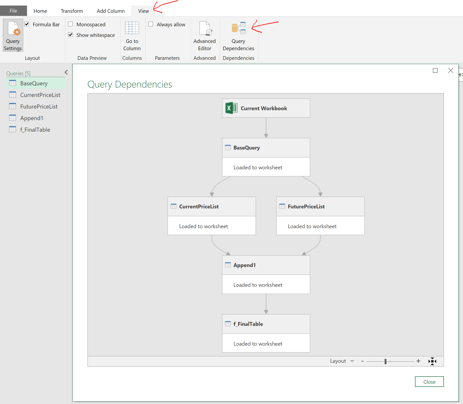
Without a single formula on Excel worksheet, we have just achieved something amazing. Most actions performed in Power Query Editor were Click and Select, with just one modification in formula bar to fix the hard-coded date filtering (which may require a bit  of Googling).  And the result is totally Refreshable when data is updated / changed.

Of course, we need to examine the data pattern and think about the logic required to achieve the end result, which require some serious thoughts.  Nonetheless, we will need to do the same via regular Excel approach.

I always tell my friends that if you can manage all the commands from Power Query’s User Interface, you are already a SUPER POWER User of Excel.  Unfortunately, they have no idea of what I am talking about, without seeing it.  That’s the motivation of this post.

Extra

Well, we have already turned a time-consuming task that may take up hours of work (if not days) into seconds.  We should be happy and complain no more.  Nevertheless, there are still rooms for improvement in terms of efficiency.

Do you remember we have modified the steps of Filtered Rows as below?

You can imagine, the evaluation of getting today takes place to each row.  We knew that in Excel, we would put TODAY() in a cell, say A1, then reference to A1 for today wherever needed.  In this way, TODAY() gets evaluated once only.

Following the same logic, we would like to revise the formula into something like:

However it would not work until we have created a query to retrieve today.

To achieve this, we start with a Blank Query, Type the following formula, Rename the Query as Today.

=Date.From(DateTime.LocalNow())

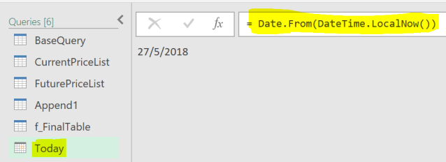
Did you notice that in the Sample File – Maintain Price Book Using Power Query (Finished), I have already created “Today” for you, so that you may revise the steps of Filtered Row directly.  🙂

How efficiency it is?

For a small dataset in our example, it makes no noticeable difference.  For a dataset of 200k rows of record, the refresh time run on my computer was about 15s.  With the slight improvement, the refresh time reduced to ~8s.  So why not?!

EndNote:

If you are new to Power Query, you may not fully understand the steps list above thoroughly.  That’s ok.  The purpose of this post is to show you what Power Query can achieve instead of giving a fully-explained tutorial.  Hopefully this post will arise your interests (and curiosity) to learn more about Power Query.

If you are expert in Power Query, I believe you may have more advanced ways of using M code to solve the problem.  If you have suggested solution in other approach(es), please share in comments.  🙂