Lookup from Right to Left

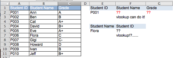
In the above example, if it is given the Student ID, it would be so easy to find one’s corresponding Name and Grade by using vlookup.  However, if we would need to find out the Student ID from one’s name, vlookup fails to help… 😦

I hope my previous posts help you understand vlookup a bit more.  You may be aware of a drawback of vlookup: the direction of the lookup.  It ALWAYS lookups the value from the LEFTMOST column in the table, then return the corresponding value X column(s) to the right.  vlookup CANNOT return a value that is on the LEFT of the lookup value.

(Yes, actually you may do left hand vlookup with CHOOSE function which many websites have described it.  However, I find that too complicated for majority users.  Moreover, I prefer simplicity to difficulty! Index and Match is definitely a better option comparing to vlookup and Choose.)

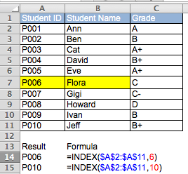
For this example, we know that Flora is the 6th value under Student Name. Her Student ID then the 6th (corresponding) value under Student ID.  In other words, we need a formula to get the 6th value under Student ID.  Here we come the INDEX function.

INDEX Functions 

There are actually two INDEX functions; one is array, the other one is reference.

Syntax

INDEX(array,row_num,column_num)
INDEX(reference,row_num,column_num,area_num)

The more I learn about INDEX, the more I am fond of it. 🙂 Indeed, if you can master INDEX, you will be an Excel guru to most ordinary users.

Nevertheless, for the sake of using INDEX together with Match as an alternative to vlookup, we can start with the basic of INDEX:

INDEX(array,row_num,column_num)

Let’s confine the array in one row or column only.  In this way, we need to input only 2 arguments for the INDEX which is really easy to understand:

For Example:
=Index($A$2:$A$11,6) simply asks Excel to return the 6^th value in the array of A2:A11

In our example, the result is “Flora”.

Therefore, if we know the relative position of “Flora” under Student Name (which is 6), then we should be able to get the corresponding Student ID of Flora easily.

Now you may have the question: How do I know the relative position of Flora?

Still remember the Match function we discussed before?

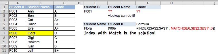
By using Match

=Match($E6,$B$2:$B$11,0) where

• E6 is the lookup value, i.e. “Flora”
• B2:B11 is the array that holds the Student Name
• 0 means Exact Match.

By substituting this Match Function into the Index Function, we will get:

=Index($A$2:$A$11, Match($E6,$B$2:$B$11,0))

The result will be “P006” which is the Student ID of Flora.  See it is exactly a lookup from right to left!

Other topics about vlookup:

1. The basic of vlookup
2. Tips in constructing vlookup
3. vlookup with Match 
4. vlookup options – True or False?
5. Advanced vlookup – Text vs. Number
6. Advanced vlookup – Wildcard Characters “?” and “*”
7. Alternative to vlookup – Index and Match
8. Three different ways to do case-sensitive lookup