It is not uncommon to work with dates in Excel.  Be it a Gantt chart for project management, a roster, or simply a calendar, we would like Excel to highlight non-working dates.  One of the most common tasks should be highlighting weekends and public holidays.  It could be a tedious manual task when you need to maintain it on monthly basis.  The good news is this tedious, boring task can be done by conditional formatting with ease.

Leave the boring tasks to Excel, enjoy your life more. 🙂 

The formula to identify day of week

On top of my mind, there are two functions to achieve this:  TEXT and WEEKDAY.

Indeed, I prefer to using TEXT function as the result it returns is more intuitive.

=TEXT($A2,"DDD")
'where A2 resides a date (input as numeric date not text)

See below to find out what I meant “more intuitive”.

Agree?

The formula for the conditional formatting to highlight weekends

We will need a formula to set up the condition.  And the formula is also intuitive:

=TEXT($A2,"DDD")="Sat"
'Note: The column is an absolute reference while the row is relative - $A2

To set up conditional formatting with this formula, follow these steps:

1. Select the range (A2:G11 in our example)
2. Go to Home tab
3. Conditionally Formatting
4. New Rule…

When the “New Formatting Rule” dialog box opens:

1. Select “Use a formula to determine which cells to format”
2. Input the formula =TEXT($A2,”DDD”)=”Sat”
3. Set the Format you want (when this condition is met)

There we go…

The row of Saturday(s) is highlighted. Yeah!

To highlight also Sundays, repeat the above steps with the following formula:

=TEXT($A2,"DDD")="Sun"
'Note: The column is an absolute reference while the row is relative $A2

Then you should get the following result:

Now let’s examine what conditions have been applied:

You will see:

1. Rule (applied in order shown): There are two rules – based on the formula we set (note: if you have more rules, you will also see them here)
2. Format: The Format set when the rule is met
3. Applies to: The range where the rule and format are applied to

Tip: Since we want to highlight both Saturdays and Sundays with the same format, we may combine the two rules into one by using the following formula:

=OR(TEXT($A2,"DDD")="Sat",TEXT($A2,"DDD")="Sun")
'Note: The column is an absolute reference while the row is relative $A2

The function OR instructs Excel to return TRUE when either one of the conditions is met.

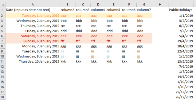
To highlight public holidays

To achieve this, we have to list the public holidays on the spreadsheet.  (Different regions have different public holidays… and the real obstacle is different industries may have different holidays, so Excel doesn’t have a built-in function to identify public holidays).

In our example, the Public Holidays is listed on $I$2:$I$18

The formula for the conditional formatting to highlight public holidays

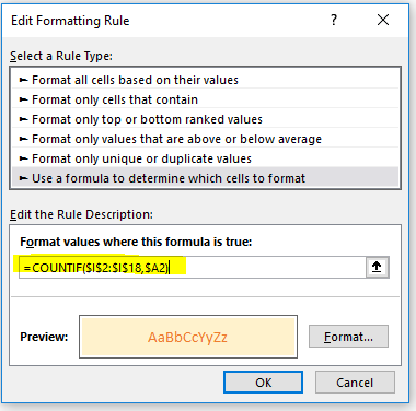
=COUNTIF($I$2:$I$18,$A2)
'Note: Pay attention to $

This formula counts the occurrence A2 (date) in the range $I$2:$I$18 (public holidays).  In other words, if it is a public holiday (as listed under PublicHolidays), it returns 1 (TRUE).  If it is not a public holiday (not listed under PublicHolidays), it returns 0 (FALSE).  This is exactly what we need to set up the conditional formatting. 🙂

Let’s add this rule by repeating the steps with the formula:

(Note: A different format is applied for Public Holiday to demonstrate another concept, which I am going to explain)

Here we go!

Let’s test it by changing the dates in column A

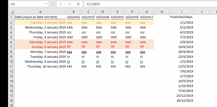
Yessssss… it’s working like a charm! 🙂

Question: What if a public holiday happens to fall on Sat?  Which formats would it display?

For demonstrating purpose, I’ve marked 2nd of March (Sat) as a public holiday.  And you may expect it be highlighted as public holiday, which is true.

Let’s examine the order of the rules set in conditional formatting:

Please pay attention to what is highlighted in Yellow in the screenshot above.

What if we switch the order of the two rules?  Watch this:

See?!  The order of rules makes a difference when there are overlapping.  First-come-first-served. 🙂

Please feel free to download a sample file to follow along and practice.  During the practice, you will find…

Conditional Formatting with formula could be tricky (or difficult), especially when the data layout is bad

because you have to very clear and careful on the “applied to” range and the absolute/relative references set in the formula.  Otherwise, it won’t work and can be quite confusing, if not frustrating.  😛

In the next post, I will talk about a case that you will see a slight change in the layout (see below) would make a difference in the set up of the conditional formatting.

where a blank row is inserted between each data for whatever reasons…

Stay tuned!