when the starting point is a negative number…

Calculating CAGR is not difficult, all we need is the starting value, ending value and the number of periods.  Then we use the formula:

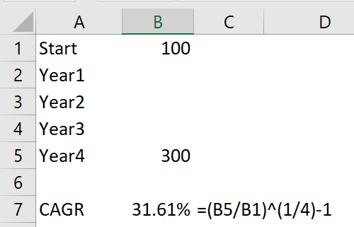
CAGR = (Ending Value / Beginning Value ) ^ (1 / N) -1 
where N is the number of periods to reach the ending period

CAGR stands for Compound Annual Growth Rate.  The formula does not require any values in between because it does not matter.  It is a “backward” calculation for the “average” annual growth with known figures.  In other words, if I have $100 on the first year and it magically becomes $300 by the end of the fourth year , and CAGR will be: 31.61%.

To validate if the result is correct, I work “forward” by calculating the value of each year by applying the growth rate of 31.61%.  We can do it in Excel easily:

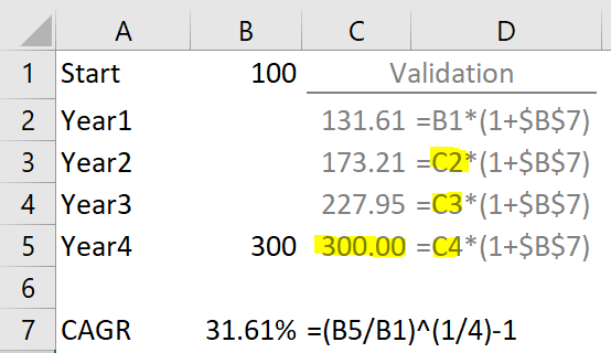
Note: the second formula (in C3) is referencing to C2, not B1.  From C3, you may copy the formula down.

I always do this kind of validation in order to double click the result.  I am not in doubt with the formula (which has been proven correct); I am in doubt with myself… As human, it’s so easy to make “human” error.

Well, the validation gives me peace of mind by returning consistent results, even with different values input…

Everything works fine until…. a negative value is input:

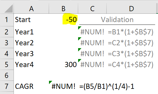
Well, if you are a finance (or math) people, you may pinpoint that CAGR cannot be computed from a negative starting value… we should start from first positive value and adjust the number of period accordingly.  Totally agree.

However, in real world situation, the requester (probably your boss) is not a finance nor a math people.  S/he just gives you three values and asks for the answer.  So the question is: Can we still do the calculation is an efficient way with Excel, when the starting value is a negative number?  Of course.

Goal Seek comes to rescue.

You may download a Sample File to follow along.

Since we cannot do it the “backward” way, we need to set up the calculation in the “forward” way.

1. In B7, I input any percentage as the constant growth rate (20% in this example)
2. In C2 to C5, I input the formula to get the values for the constant growth rate year on year.

Note: instead of using the commonly used simplified formula, i.e.

Value * (1 + growth rate)

I have used the traditional way with a slight modification – wrapping the value with ABS to tackle the negative values we may encounter.

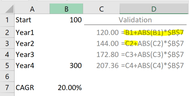
In C2, the formula is

=B1 + ABS(B1)*$B$7

Also note the formula in C3 is referencing to C2, not B1.  You may copy down the formula from C3.

Make sense?

If that makes sense to you, you should have known the next step now… 🙂

Change the value in B7 manually in order to set the value in C5 to 300.  Like the following screencast:

If you are super lucky, you may (if you could) get the answer by trials and errors… Well… if you are super lucky, I have to repeat. 🙂

Goal Seek comes to rescue

• Go to Data Tab –> What-If Analysis –> Goal Seek

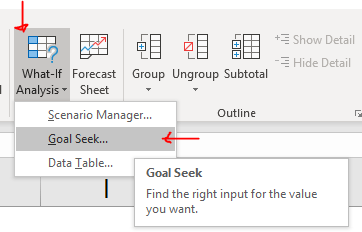
• Input the three parameters as shown below:

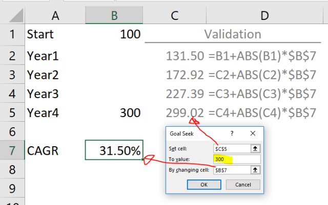
In plain English, it means: Excel please sets the value of C5 to 300 by changing the value in B7.

Straight forward.  Isn’t it?

• Sit back and watch Excel does the job for you!

WOW!!!  Goal Seek found a solution!

Needless to say, we are going to change the starting value (in B1) to a negative number and repeat the Goal Seek steps above:

As simple as this.

With Goal Seek, we found that the “Constant” yearly growth rate we need to grow a value from -50 to 300 in four years is 142.22%.

Can we still called it CAGR?  well… I don’t know.  And worse still, the result would be paradoxical.  Why?  Try with few negative numbers from larger to smaller values.  You will see that the smaller the starting value, the lower the constant growth rate requires to reach a fixed ending value.  Quite confusing…

Nevertheless that is not the topic of this post (or this blog).  I just tried to show you what Goal Seek does.  🙂

If you know the correct way of calculating CAGR with a negative starting value, please share your thoughts in comments.