This is a real workplace problem.

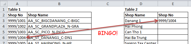
Look at the two tables below, the task was to map the Shop ID from Table 1 (left) to Table 2 (right).  In both tables there is a common key “Shop Name”.  Sound easy? Pls look at the tables first.

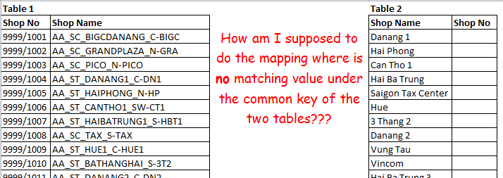
The so-called common key appears to be totally different in the two tables.  How could it be possible to do the mapping by formula when the values in the common key are so special??

If not by formula, was I supposed to do that manually by eye-balling?  (The list is much long than what is shown above… ) That stopped me for a second look at the tables again.  Thanks GOD, there is one “commonality” in the “Shop Name”.  Do you see?

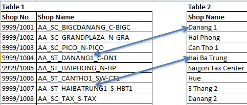
In Table 2, when all spaces in shop names are taken out, we see the “Shop Name” somewhere in the middle of the “Shop Name” in Table 1.  I see light in the darkness because the task can be done by formula and be completed in just a minute…  How? Let’s do it step by step.

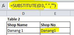
Step 1 – Remove “Space” in the lookup values by using function SUBSTITUTE

The Sytax

=Substitute(Text,Old Text,New Text,[instance number])

In the example, it simply means: Look at the text in “D3”, substitute space (” “) with nothing (“”).  As [instance number] is omitted, Excel will substitute all spaces found.

Result: “Danang1”

Step 2 – Add “*” in front of and after the above result by using “&” for subsequent lookup

The “&” operator serves the same function as CONCATENATE.

Now the result is: “*Danang1*”

Note: * is a wildcard meaning text string of any sequences.

“*Danang1*” now serves the purpose of looking up from Table 1.

Step 3 – Identify the relative position of the above result under Shop Name in Table 1

The Syntax

=MATCH(lookup_value,lookup_array,match_type)

In this example, the lookup_value is the result in Step 2 that is “*Danang1*“.  Literally the formula means: Look up any text that contains “Danang1” in between, from the range of B3:B100 where holds the Shop Name in Table 1.  Once a matched value is found, returns the relative positive in the range.  Exact match pls.

Result: “4″ 

Step 4 – Get the corresponding Shop Name by using INDEX

The Syntax

=INDEX(array,row_num,column_num)

It simple means in our example that under “Shop No” (A3:A100) in Table 1, return the 4th value.

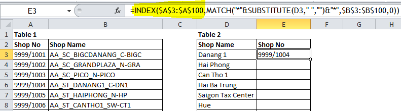
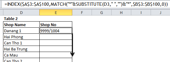
This is the final formula:

=INDEX($A$3:$A$100,MATCH(“*”&SUBSTITUTE(D3,” “,””)&”*”,$B$3:$B$100,0))

Result: “9999/1004”

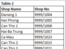
Step 5 – Get the job done by filling down

Result:

Final Step – Relax and enjoy a cup of your favorite drink

If you were me, would you submit the result to your boss immediately?? 😛