
Don’t make me wrong. I am not complaining Power Query at all. If you have followed me for a while, you should know that I am a big fan of Power Query indeed. It is simply powerful! With Power Query, lots of data cleansing, reshaping, consolidating tasks become easy and efficient. If you want to learn more what Power Query could do, have a look at my blogposts and playlist of videos related to Power Query.
To me, data cleansing is a process with seven stages:
- Understanding the expected outcome
- Studying the data on hand
- Finding the pattern(s)
- Cleansing the data (this is the stage most people interested in)
- Checking the results
- Refining the cleansing steps (most of the cases required, and need to go back to stage 2)
- Repeat the above cycles until the expected outcome is obtained
Most of the time, we focus on stage 4, i.e. Cleansing the data itself. Nevertheless, stages 5 to 7 are critical to success, although often got unnoticed.
Let me show you an example here. (Note: this post is not a step-by-step tutorial).
Situation
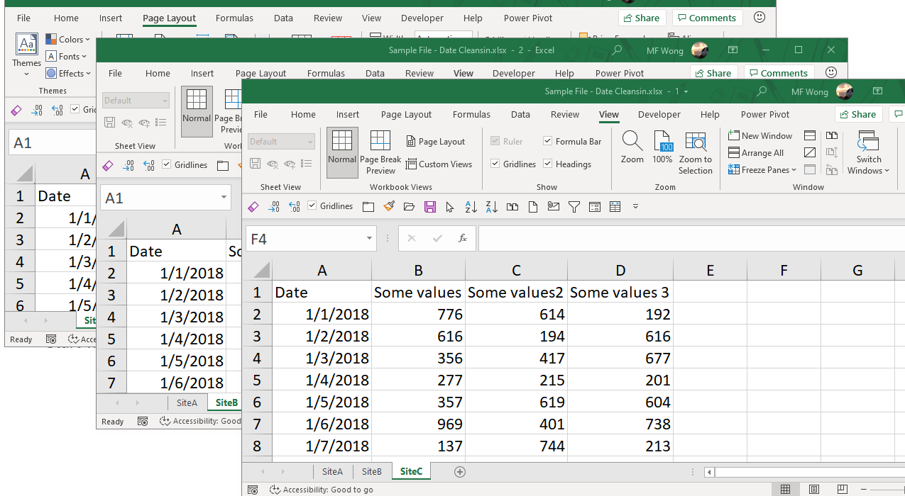
I was presented with a few Excel workbooks. On each worksheet of each workbook, it holds daily sales data of a location. I was told that all worksheets across different workbooks are “exactly the same” in layout and structure.
Stage 1 – Understanding the expected outcome
The task is to consolidate all data into one single table showing daily records by location, like this:

Well, if you know Power Query, you may think that this task is not difficult at all, probably easy indeed…
Stage 2 – Studying the data on hand
As I was told that every worksheet is the same in layout and structure, I focused on one worksheet to study the data. Here’s my findings:
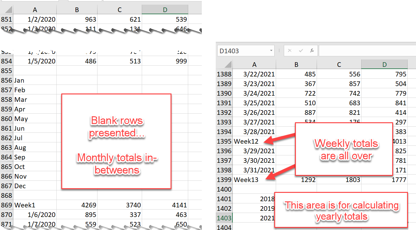
- Blank rows are presented
- In the middle of the sh*t, there are weekly and monthly subtotals (how typical, isn’t it?)
- All the way down, there are also yearly totals
- The last used cell sits on row D1403
(Tip: always jump to the last used cell by using Ctrl+End whenever dealing data stored in Excel)
Stage 3 – Finding the pattern(s)
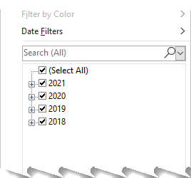
As the information on column A is crucial for the cleansing task, I decided to select the entire column and apply a filter on it, so that I could see everything under column A:

(Tip: Under normal circumstance, do not select the entire column(s) for filtering as it intakes unnecessary rows)
I had clear visual on column A. It has dates, numbers, and texts, and blanks. What I needed was only dates. Not too bad. First thing on top of my mind was to set the data type to “Date” for column A, so that everything else would return “error” which I could easily remove subsequently.
In short, my first query plan:
Convert Column A into Date ->
Remove Empty and Errors
Stage 4 – Cleansing the data
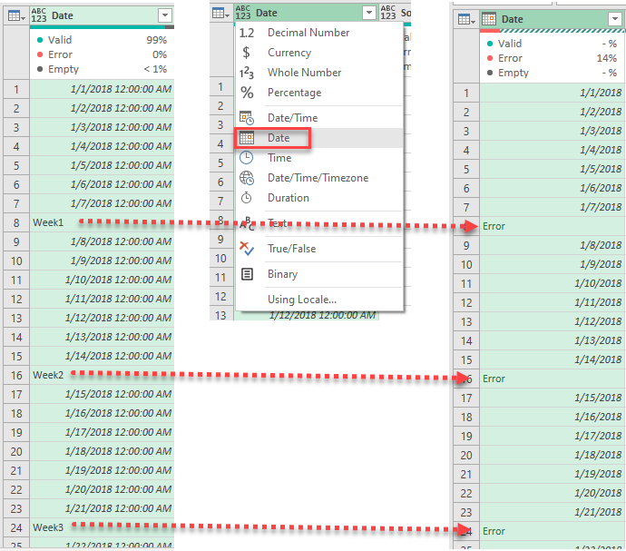
When I defined data type in a column in Power Query Editor, I’d got “Error” when Power Query failed to convert the data into the data type specified. In our example above, “Text” could not be converted to “Date“. As a result, “Error” was returned, which I could remove them easily afterward.
By doing so, I was essentially removing all text values.
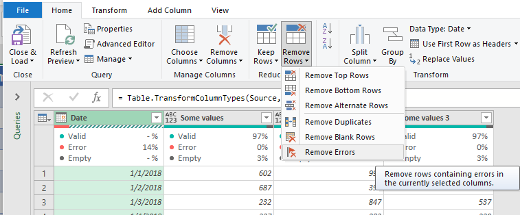
Next step would be Remove Empty:

Cool! I had removed all “texts“, “null” and “blanks” already, as planned.
Let’s have a look at the data being filtered:

Stage 5 – Check the results
Apparently, all dates remained which is good but somehow I felt something wrong. The ⚠ sign “Limit of 1000 values reached” was telling me that I was reviewing only part of the data. So I loaded the data to a worksheet to exam.

What? Why there are data back to July in 1905? 🤔
Do you remember that at the bottom of each sh*t, there are rows for calculating yearly totals?

The presence of numbers in column A breaks the pattern. These numbers will be converted into “date” when I set the data type to “Date“.
Note: Excel stores dates as sequential serial numbers so that they can be used in calculations. January 1, 1900 is serial number 1, and January 1, 2008 is serial number 39448 because it is 39,447 days after January 1, 1900. You will need to change the number format (Format Cells) in order to display a proper date.
From: Microsoft Support page
As as result, 2018, 2019 and 2020 are converted into 10th, 11th, 12th of July in 1905 respectively. That’s why.
Stage 6 – Refine the cleansing steps
Luckily this is not a big deal because there is a clear pattern for these numbers. These numbers are “Year”. It means they will always be a four-digit numbers (or even two-digit numbers) in my life. It will never fall into any valid date range in my dataset (on which the earliest date is the first day of 2018). After finding this pattern, I modified the query by adding a filter step (Date is after or equal to 1/1/2018) at the end in order to exclude those numbers.

Then I loaded the data and check again.
Bingo! Thus I turned the cleansing steps (query) into a function so that I could apply the same set of cleansing steps to different worksheets across workbooks in a folder. You may read this post or this post if you want to learn more about the related topic.
Stage 7 – Repeat the above cycles until the expected outcome is obtained
With Power Query, the cleansing and consolidating tasks took only a few seconds to execute (Stage 4). Simply Powerful! But the task was not yet done. I had to check the result again (Stage 5). Yes, again… and you will see why very soon.
Given my dataset, an easy checking point would be the number of records by location by date. There should be only one record per location per date. However, real life is not that easy…

Surprisingly there were duplicated records found for SiteB. And the interesting point was that the duplicated values only happened on the first date of each month while the duplicated records showed a BIG number. What was going on?
So I double-checked the data on SiteB carefully. I was pretty sure that there were no duplicated dates on the dataset. Each date appeared only once. What could be wrong???
I scrolled down the sh*t row by row….. Wait…
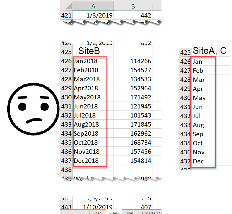
Somehow, the row headers for the monthly totals are different on this sh*t. In other sh*ts, these are only month names, with no year associated to it. But for SiteB, a four-digit year numbers were added to the month names.
This breaks my sample query perfectly!
You may be surprised why?
Let’s go to the Power Query editor and see what happened when I tried to convert these texts into date:
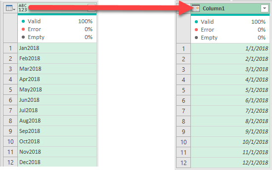
This is exactly the reason we got duplicated records for just the first date of each month.
To most users, this is an unexpected and undesired result. Indeed, this is kind of a feature for Excel to “guess” what user intended to input. You may want to learn more from this post – What we need to know about inputting Date in Excel?
Because of this slight inconsistence in data, my original query plan didn’t work for the entire dataset. It worked just for SiteA and Site C, but not for Site B. (Again, this is a simplified version. In real case, there are many more worksheets in multiple workbooks)
Therefore I had to find another pattern that would work for both cases (Stage 6). After a closer look at the dataset (in multiple sample sheets), I came up with a new query plan that worked well in my case.
Here’s the new (and final) query plan:
Convert Column A to Text -> Keep rows that contains “/” (a good indicator of date) -> Change data type to Date
The cycle looped again… and this time I was happy with this pattern. The entire dataset got cleaned and consolidated; nothing missed nor duplicated. 😁
Conclusion
I am not saying that the final query plan is bullet proof. Indeed, it is not. It is just good enough for my dataset.
Nevertheless, the key point is not the solution itself. It is the entire process.
With Power Query, the data cleansing tasks have become (relatively) easy. When we learn Power Query by reading tutorials or watching YouTube videos, our attention might be drawn to the execution part. That’s normal. After we start picking up the skills of Power Query, we will find that the difficult part is not necessarily the cleansing tasks itself, but finding the patterns and hence solutions that fit different scenarios.
In case you would like to try, you may download a sample file below:


