Combine all visible worksheets from multiple #Excel files in a folder

It is a common task for us to combine all worksheets in a workbook. It could be a time consuming task without Power Query. With Power Query, it’s piece of cake. 😁

Wait? What about if you want to combine all visible worksheets from all Excel files in a folder? It requires a little more Magic from Power Query but it’s totally achievable without deep-diving into M code… just touching the surface would do. 😉

Let’s watch it in action:

You may download the sample files HERE to follow along:

(note: suggest you put the Q4 file aside for “refresh” later)

Step-by-Step instructions with screenshots

If you prefer reading to watching, please continue to read the step-by-step instructions below.

Open a blank Excel workbook.

Go to Data tab
Get Data
From File
From Folder

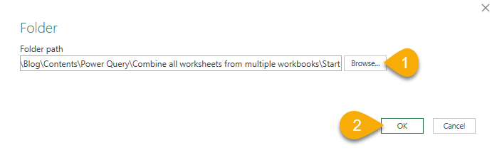
Browse the folder where you have the Excel workbooks for consolidation
OK

Open the pull down for “Combine” ==> Combine and Transform Data

(Note: In earlier versions of Excel, you may see it as "Combine and Edit")

Right-Click the “Parameter1”
Select Transform Data (or Edit)

At this point, the Power Query Editor opens with all the information from each workbook loaded into it.

Since all tables on worksheets across different workbooks follow exactly the same layout and structure, we may apply the same set of transformation steps to all the tables involved.

A sample table is needed to record the required transformation steps before we combine all the tables. Let’s use the first table as sample table.

Right-Click on an empty space next to the first table
Select “Add as New Query”

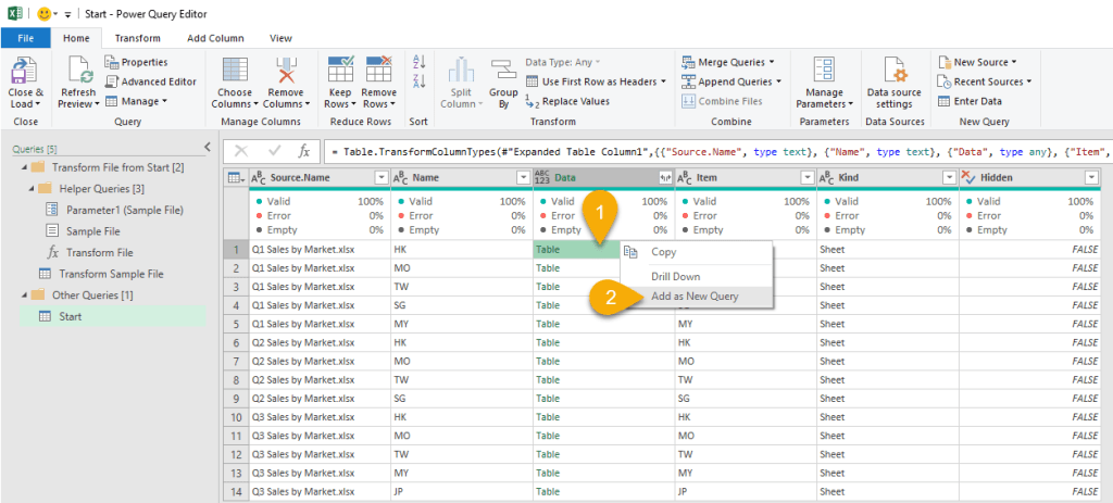
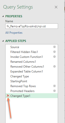
A new query “Data” is added. Let’s rename the query name as well as the last step of the query.

Change the query name from “Data” to “fn_RemoveTopRowsAndUnpivot” (because I am going to remove unwanted rows and then unpivot the table in order to normalize the column names on each table. After all, I will convert this query to a function that will be invoked later.)
Change the last step of the query from “Data1” to “StartingPoint“

After the renaming, you should see the below in the Query Settings Pane:

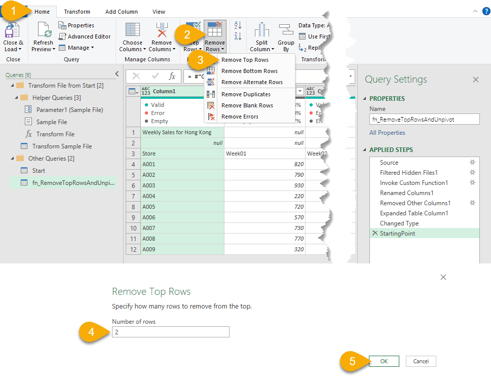
Let’s do the first transformation – remove unwanted rows

Go to Home tab
Remove Rows
Remove Top Rows
Input 2 as the number of rows to be removed (as our tables start on row 3)
OK

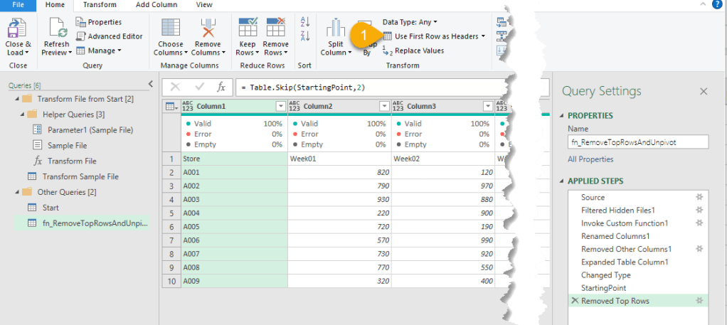
We are now ready to promote the first row as headers

Click the “Use First Row as Headers” on the Home tab

After this “Promote Header” step, a step “Change Type1” is generated automatically by Power Query. We don’t want this step. Click the ❌ on the left to remove it.

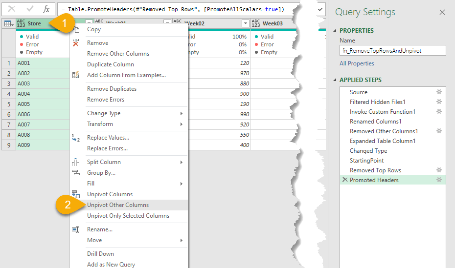
Now we are ready to UNPIVOT the table to normalize all the columns headers. Why we need this step? Think about the fact that there are different columns headers in different files. For Q1 file, we have headers of Week01 to Week 13; while for Q2 file, we have headers of Week14 to Week26. And so on and so forth.

Because of this, we cannot directly “Append” the tables together as each column hold sales amount of different periods. Therefore, we need to UNPIVOT the tables to make sales data of all “weeks” to be fallen on a single column (attribute).

To UNPIVOT

Right-Click the anchor column “Store”
Select “Unpivot Other Columns”

You won’t believe how easy it is to unpiovt a table with Power Query. BUT IT IS! 🙂

Let’s rename the “Attribute” and “Value” to “Week” and “Sales Amt” respectively. (by double-clicking the header and then rename)

Now under the column “Week”, the word “Week” in the data is abundant. We can remove it by using “Replace values”.

Select the column “Week”
Go to Home tab
Click “Replace values”
Input “Week” in the “Value To Find”
Input nothing under “Replace with”
OK

In plain English, the above steps instruct Power Query to replace the word “Week” with nothing in the “Week” column. Make sense?

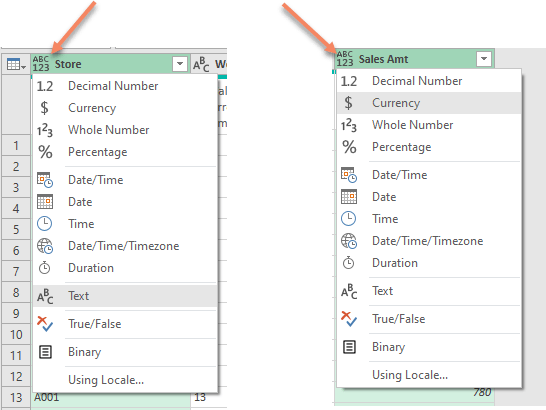
Let’s define the data type accordingly!

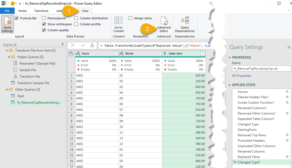
Take a look at the Query Settings pane. These are the six steps we performed to the sample query. And these six steps are all we care about; these six steps will be applied to tables in all the Excel workbooks in the folder.

To convert these six steps into a function for later use, we need to open the Advanced Editor.

Go to View tab
Select “Advanced Editor”

Don’t be scared by the codes in the Advanced Editor. At normal circumstance, each line of code represents each step you see on the Query Settings Pane. And these codes are generated automatically by Power Query. At this point, we don’t have to know all the functional codes here. We just need to identify the codes where the six steps we want. Everything else under the “let” statement can be deleted.

These are the codes of the six steps we want.

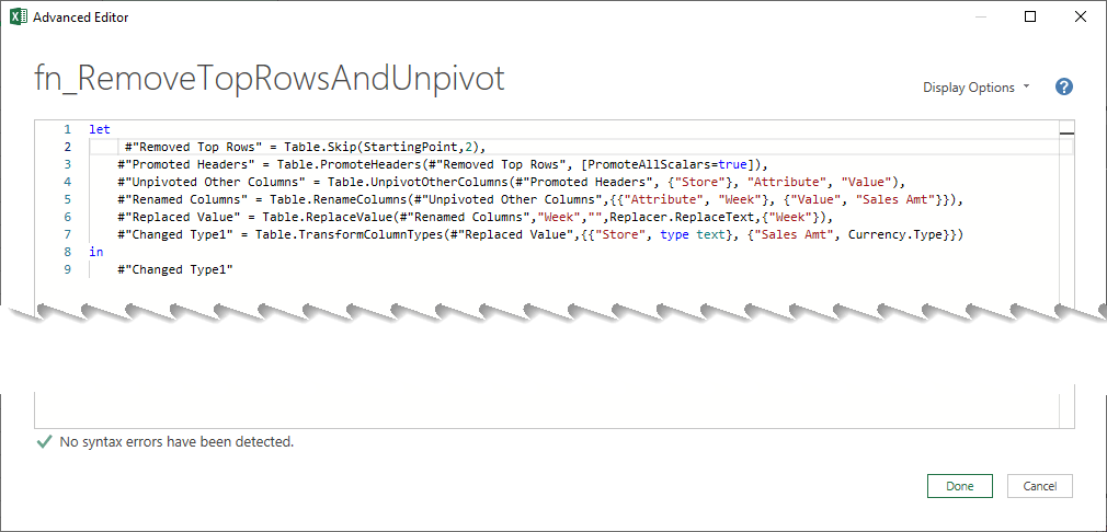
To turn these steps into a function, we need to input the following on top of the let statements. On the first row, insert:

(StartingPoint as table) =>

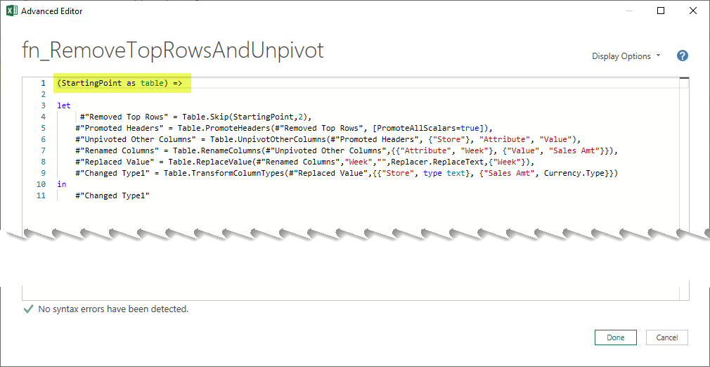
Why “StartingPoint as table”?

Because that is the parameter (table) being fed into the first step Table.Skip(StartingPoint,2)

When it is DONE, we see that Power Query turns the query into a function which we can call for later.

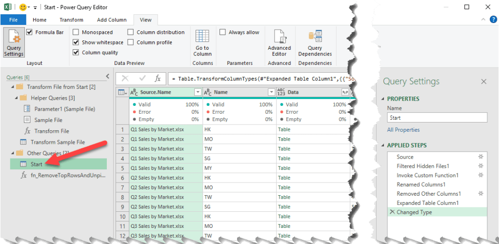
Now, we are ready to apply this custom function to the “Start” query.

Select the “Start” query

Keep the columns we need.

Select both “Name” and “Data” (where name is the worksheet name that happens to be the market name. I want to keep this information. Whereas “Data” resides all the information we need as table).
Select “Remove Other Columns”

Rename “Name” to “Market”

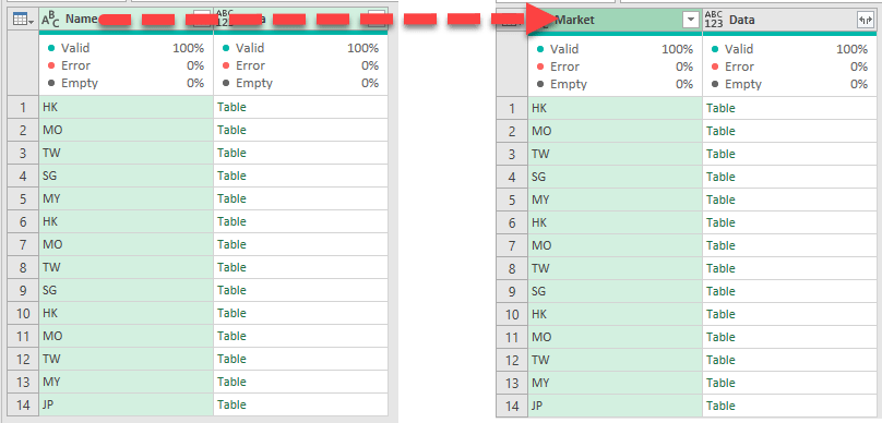
At this point, we should have kept only two columns:

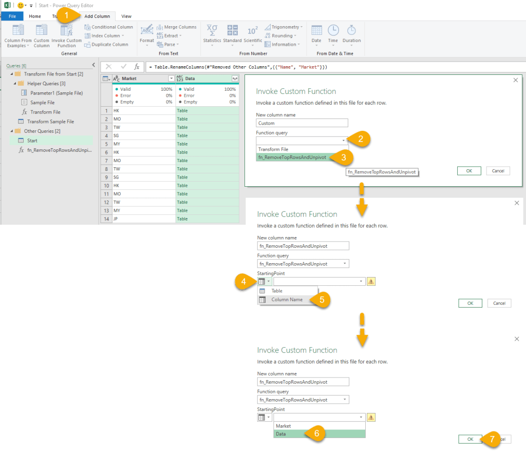
To Invoke the function to all the tables under “Data”

Go to Add Column tab –> Select Invoke Custom Function
Open the pull down for “Function query”
Select “fn_RemoveTopRowsAndUnpivot” (that is the function we created before)
Open the parameter input option
Select “Column Name” (as we want to invoke the function to all tables in “Data” column)
Select “Data” (which is the column holding all tables to be transformed)
OK

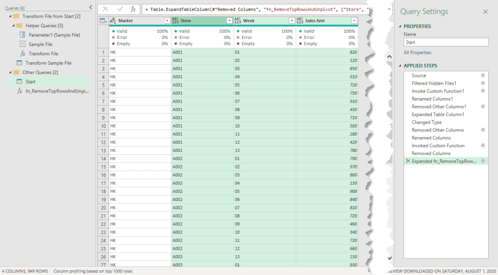
Here we go! An additional column with “transformed” table! 🤞

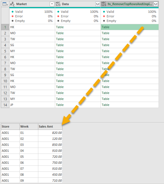
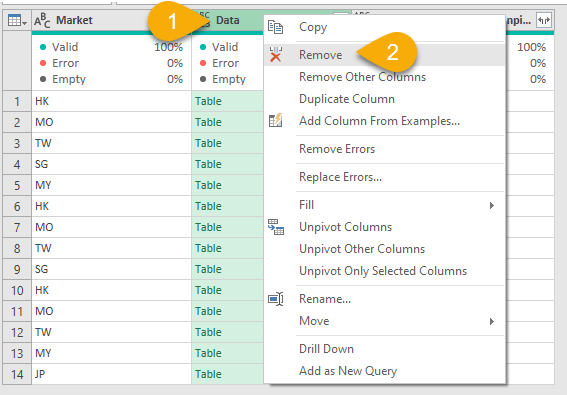
The original “raw” table can be removed.

Right-Click the “Data” column
Select “Remove”

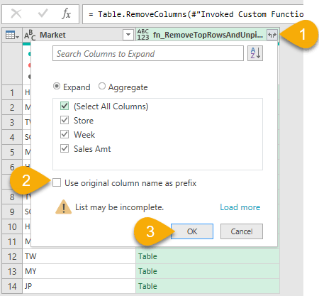
To expand all the data fields from the “transformed” table

Click on the “expand” icon
Un-check the “Use original column name as prefix”
OK

Here we go!

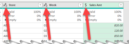
As good practice, always define data type for each columns before loading the data.

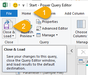
To load the result to worksheet

Go to Home tab
Click Close & Load

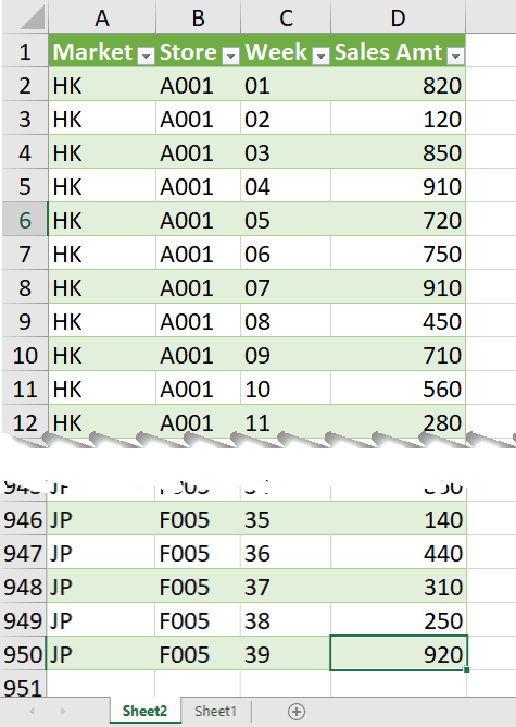
Here’s the consolidated data; with all the data from all worksheets in each Excel workbook in the folder! Amazing!

Wait… the title of this blogpost is