Well… think this topic is too simple?  How about doing this with

1. a dropdown menu to make the Top X a dynamic one?
2. with Icon Set?

You may download a Sample File to follow along.

Let’s start with the basics first.  Here is

The simple way of highlight Top X

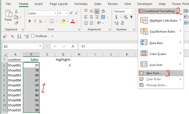
1. Select the range of data (where you the conditional formatting applies to)
2. Go to Home Tab –> Conditional Formatting
3. Top 10 items…
4. The select the Top X (tip: you can customize the format)

Super easy!  Indeed it is a very handy way to highlight Top X values in a dataset.  The only drawback is the Top X is statics.  If you want to change the number of values to be highlighted later, you need to go deep into the conditional formatting to revise the Top X value:

1. Conditional Formatting –> Manage Rules…
2. Select the rules –> Edit Rules…
3. Change the value, then OK, OK

This slideshow requires JavaScript.

Not quite ideal…

So why don’t reference the (Top) X to a cell, say G2, where a user can input directly?

Like this:

Ooops…..

I hope the above would work… but it is not that easy.  Sometimes Excel prefers to giving you hard time, or challenge (be more positive). 🙂

To achieve this, we need a workaround to build the conditional formatting rules by using formula.

Setting the condition using a formula

A) Setting up New Rule for conditional formatting:

1. Select the range of data
2. Home tab –> Conditional Formatting
3. New Rule…

B) Define the condition by a logical formula:

1. In the dialog box of “New Formatting Rule”, select “Use a formula to determine which cells to format”
2. Input the following formula:

=B2>=LARGE($B$2:$B$11,$G$2)

‘Note: Pay attention to the relative and absolute references.

3. Click “Format…” to set the format you want

C) Setting up the format when the condition is met

1. Go to the “Fill” tab
2. Select the Fill Color that you want
3. OK

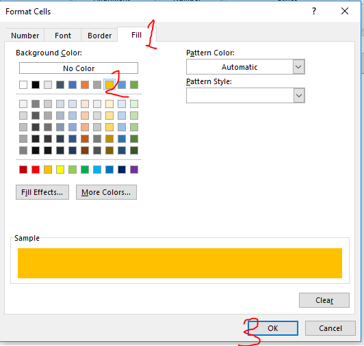
Tip: You may set other formats in the other tabs

All set.  Let’s see the result:

How this work?

Let’s examine what the formula does.

=B2>=LARGE($B$2:$B$11,$G$2)

Syntax – LARGE(array, k)

• Array    Required. The array or range of data for which you want to determine the k-th largest value.
• K    Required. The position (from the largest) in the array or cell range of data to return.

In a word, to return the Top X value.

The LARGE($B$2:$B$11,$G$2) returns the Top X value in the range of $B$2:$B$11, where X is the value in $G$2.  This result is then compared to the value in the range by the following portion:

=B2>= Top X value

In short, the formula compares the cell values to the Top X value in the range, to see if the cell value is larger or equal to the Top X value.  When it is TRUE, then the format is applied.

Put it into other words, it is the formula expression of the Top X rule of conditional formatting.  Make sense?

Let’s make a dropdown in G2 to make it interactive

1. Select the cell G2
2. Go to the Data tab
3. Select “Data Validation” on “Data Tools” group
4. Select the “Settings” tab (selected by default)
5. Select “List” under “Allow:”
6. Input 1,2,3,4,5 under “Source:”
7. OK

Note: Make sure the In-cell dropdown is checked.

Now you will see the dropdown button when G2 is selected.

Yeah!  All done… but one final trick…

The Final Trick

What?  Did you notice that in the first image of the post, we have “Top ” before the number when it is selected?

Using Custom Format to make a number more “meaningful”

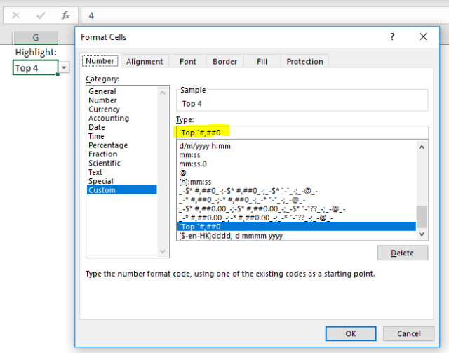
In G2, Apply the following custom format:

“Top “#,##0

This custom format adds the prefix “Top ” to the numeric input.

Important: We cannot use “Top 1”, “Top 2”, “Top 3”, etc as the dropdown directly as it will turn the cell content into Text instead of Number.  The LARGE function would not work with “text” argument.

Note: Pay attention in the formula bar.  Although you see “Top X” in G2, you see only “X” in the formula bar.

I use this trick a lot to make my worksheet more “interactive” while maintaining “readability”. 🙂

I hope you like it too.

What about doing the same with Icon Set?  well… I will talk about it next week.  Meanwhile, I highly encourage you to try and explore.  The logic behind is more or less the same.  You just need to figure out where to put the formula.  🙂