This post is a continuation of the previous one – Highlighting Top X values with Conditional Formatting in #Excel

So I will go straight to the point.  For background information, please read the previous post. 🙂

To insert Icon Set

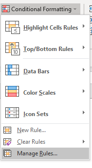
Select the data range –> Go to Home Tab –> Conditional Formatting –> Icon Sets

Choose the icon set you like.  For this demonstration, the set of flags is used.

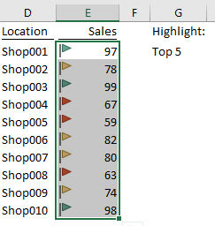
This is the result you will see.  However, we don’t want all three flags.  We just want to have a green flag for the Top X value(s).  So let’s manage it.

Modify the Icon Set and Formatting Rules

Select the Rule, then “Edit Rule…”

Here we go…

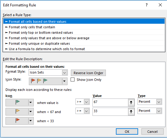
Note: The Rule Type “Format all cells based on their values” is selected by default if you have been following the steps.

Guess where we are going to modify?

… The “Icon”

… The “Value”

… The “Type”

Bingo!

Let’s watch it in action

Note: The “logical operator” selected is “>=” (larger or equal to)

This is the formula we input:

=LARGE($E$2:$E$11,$G$2)

‘What this formula does? Please read previous post

Note: Even though we have selected “No Cell Icon” for other rules, it does not mean you can leave the rules empty. Also we should not have contradicting rules set. As a simple rule, I would you select the same Type, and input the same numbers in the two value boxes. Do pay attention to the operator selected for the rules to get your desired result.

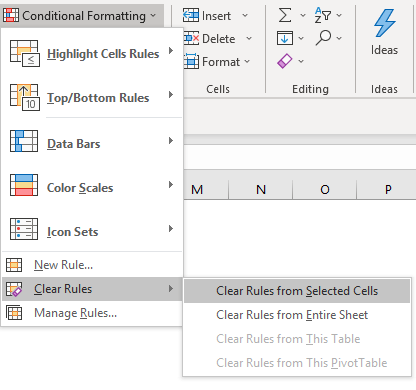
You may download a Sample File file to follow along… but you may want to clear the existing rules first.

Like it?  Please leave us comment to share your thoughts. 🙂