Transform date input as “Excel-unrecognized” text string into date (number) usable by #Excel

This is a continuation of the previous post – How to turn “1st January, 2017” into #Excel recognizable date?   …using Get & Transform (better known as #PowerQuery).

Note: All screenshots and steps in this post are based on Excel 2016.  The ribbon of Power Query for Excel 2010/2013 may be different a bit… but the steps and interfaces should be more or the same.

The problem was discussed in the previous post.  So let’s go straight to the solution:

You may download a Sample FIle – Reversed Text Date to Number Date to follow through.

Step 1 – Load the data to Power Query

Select the range of dates to be transformed, then go to

Data –> Get & Transform Data (group) –> From Table/Range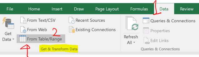

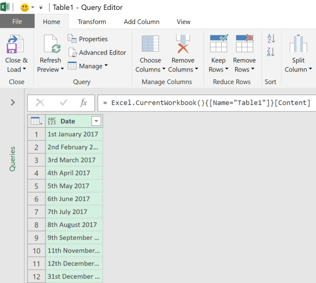
Now we have opened the Query Editor, with the data loaded into it…

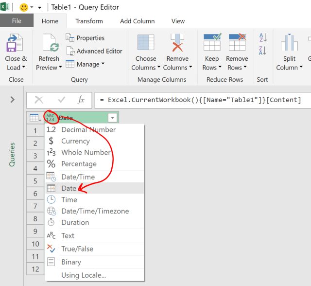
Be curious!  Let’s explore a bit by clicking the “ABC 123” icon on the column header “Date”… wow, there is a list of different data type.  It looks promising!  So I clicked on it and selected Date hoping for the magic instantly.

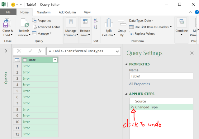
Oooooops…. all Error.

Apparently, Power Query fails to recognize this kind of “date” too.

Don’t be frustrated.  We need just a few more steps to achieve our goal.

Now, let’s undo the “Changed Type” step.  Unlike in Excel, Ctrl+Z won’t undo the step applied in Query Editor.  We need to remove the “Applied Steps” in the pane of Query Settings.  See below:

Step 2 – Split Day from Month and Year

Now let’s go to

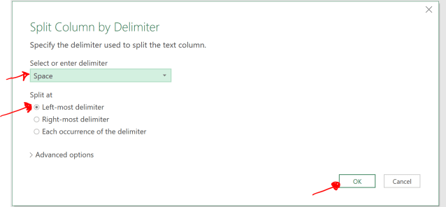
Transform –> Split Column –> By Delimiter

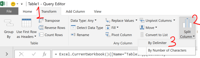
Select Space as delimiter; Split at “Left-most delimiter” as we are trying to separate the day portion from month and year…  (Think about why we need this step)

The Date is now split into Date.1 and Date.2.  And Power Query recognizes Date.2 “January 2017, February 2017, etc…” as date and automatically changes it to date… Well, this is helpful most of the time but not in our case here.  So we need to undo this “Changed Type” from “Applied Steps” under Query Settings.

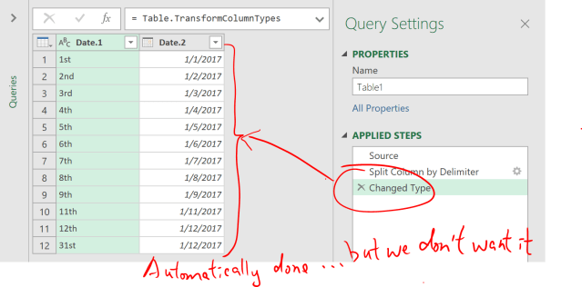
Note: After removing “Changed Type”, both columns are recorded as “text” indicated by the “ABC” icon on column header.

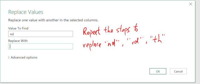
Step 3 – Replace Values

In order to remove all “st”, “nd”, “rd” and “th” from Date.1, go to

Home –> Transform (group) –> Replace Values

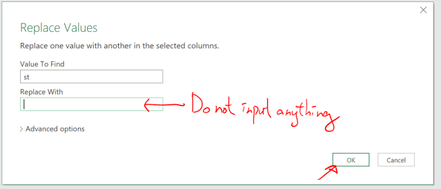
The step above remove all “st” from the column Date.1

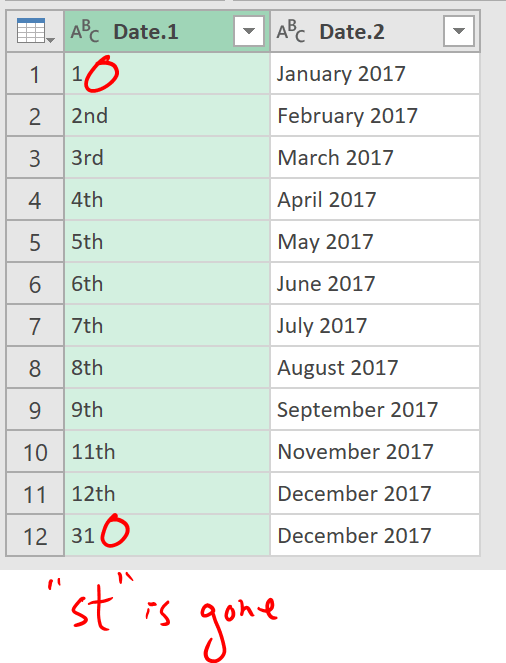
Now repeat the steps to remove “nd”, “rd” and “th”

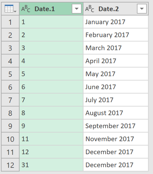
We should get the following as a result:

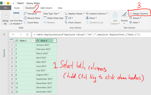
Step 4 – Combine “trimmed” Day with Month and Year

First of all, select both columns Date.1 and Date.2, then go to

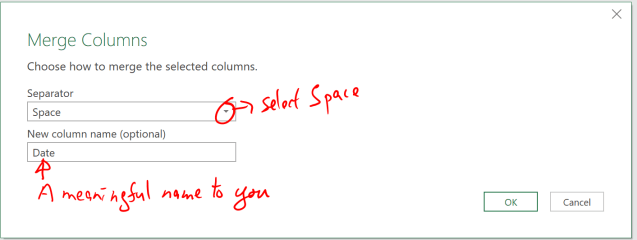
Transform –> Merge Columns

Select Space as Separator, and give the new column a meaningful name:

Step 5 – Change Type

Now the “Transformed” date is ready for changing type as it’s now in a text pattern recognized as date by Excel.

Click the “ABC” on the column header,  

Then select “Date”

Here we go…

Final Step – Load to worksheet

To load the “transformed” data back to Excel worksheet, go to

Home –> Close and Load To… —> Table –> Existing worksheet –> Destination –> OK

Output

And the best is yet to come…

When new data comes, a simple (right) click of “Refresh” does the magic:

Yes, that’s what we all do in office day by day: Repetitive and tedious tasks, again and again…

With Power Query, we can say GOODBYE to repetitive, tedious, and probably boring tasks.

You may wonder why we need to split day and then combine it with month and year later.   Why we need such extra step?  Simply because one of the replacing values “st” also appears in “August”.  If we do not split day from the month first, “August” will become “Augu” after replacing “st” and it results in error of all dates in August.  Try it and you will see.

Want to learn more about Power Query?

Disclosure: I earn a small commission if you finally take the course via my site.