
Well, there is no such custom format for date in Excel… However it can be achieved indirectly, with helper cell 🙂

Let’s take a look at the available date formats in Excel:

As shown above, there are many different “numeric” and “textual” expressions for
- Day (e.g. 1 or 01)
- Day of a week (e.g. Mon, or Monday)
- Month (e.g. 1, 01, Jan, January, J)
- Year (14, or 2014)
By arranging them with your favorite separator (e.g. space, comma, hyphen, forward slash or even a dot) in your desired order, various date formats can be customized. For instance, if you format 1/1/2014 as “dddd, mmmm dd, yyyy” will give you “Wednesday, January 01, 2014” as a result. However there is no such format for “1st of January, 2014”.
The wonderful thing about Excel is there would be often (if not always) an alternative way to achieve what you want. Isn’t it?
Suppose we have the date (say 1/11/2014) in D2, we may apply the following custom format to it:
- Format: mmmm, yyyy
- Result: November, 2014
 ==>
==> 
The trick now is to create day (with corresponding suffix “st”, “nd”, “rd”, “th”) in the helper cell (C2) by the following formula:
=DAY(D2)&LOOKUP(DAY(D2),{1,"st";2,"nd";3,"rd";4,"th";21,"st";22,"nd";23,"rd";24,"th";31,"st"})
The formula does the following:
- Day(D2) – returns the day of the month in number
- LOOKUP(DAY(D2),{1,”st”;2,”nd”;3,”rd”;4,”th”;21,”st”;22,”nd”;23,”rd”;24,”th”;31,”st”}) – returns the corresponding suffix of the day
This can be understood easily if we visualize the {green part} into a table. 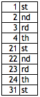
CONCATENATE them, we will have “1st”, “2nd”, “3rd”, “4-20th”, “21st”, “22nd”, “23rd”, “24-30th”, or “31st” according to the date value we have. So, here we go:

Tips: If you wish to have “1st of November, 2014” instead, apply the following custom format in D2: “of” mmmm, yyyy (the double quotation mark is required)
Extra:
The mmmmm (m x 5) is a less well-known format for Month. It formats the month into J, F, M, A, M, J, J, A, S, O, N, D for from January to December respectively.
The benefit of it: SPACE. It could be helpful in dashboard report or mini chart where real estate is expensive.
By the way, I have no idea why there is no such format for day of week… @_@


Thank you so much for this solution! Helped me a bunch!
LikeLiked by 1 person
You are welcome. Glad it helped! 😃
LikeLike
This works better:
=DAY(D2)&VLOOKUP(MOD(DAY(D2),10),{0,”th”;1,”st”;2,”nd”;3,”rd”;4,”th”},2)&” “&LOOKUP(MONTH(D2),{1,”January”;2,”February”………})
LikeLike
Hi Pete,
Nice use of MOD. However by using MOD, it gives 11st, 12nd, and 13rd while the correct expression should be 11th, 12th, and 13th.
For the latter part of the formula, it will be easier to use TEXT(D2, “MMMM, YYYY”).
Cheers,
LikeLike
This is really short & great. I did as follows.
Col. A42 = “05-10-2023”, C42 = “06-09-2023”. Ans is “10th May to 9th of”
=” from”&DAY(A42)&VLOOKUP(MOD(DAY(A42),10),{0,”th”,1,”st”,2,”nd”,3,”rd”,4,”th”},2)&TEXT(A42,” mmm”)&” to “&DAY(C42)&VLOOKUP(MOD(DAY(C42),10),{0,”th”,1,”st”,2,”nd”,3,”rd”,4,”th”},2)&” of”
Thank you.
LikeLike
This should make the trick:
=IF(ISNA(VLOOKUP(MOD(DAY(D2),10),{1,”st”;2,”nd”;3,”rd”;4,”th”},2))=TRUE,”th”, VLOOKUP(MOD(DAY(D2),10),{1,”st”;2,”nd”;3,”rd”;4,”th”},2))
LikeLike
How is the reverse possible? I mean if I have a column with dates as “1st November, 2017” how can I get excel to understand so I can apply formulas like =DAYS() etc
LikeLike
Hi Vinay
That’s an interesting question. You will need formula to fix that. Let me write a post to explain it . Stay tuned 😃
LikeLike
Have a look. See if it answers your question. 🙂
LikeLike
Super. Thanks.
LikeLike
You are welcome. Glad you like it. 🙂
LikeLike
Is this possible in Word 2016?
LikeLike
Thanks for the formua, i added some more to it.
=CONCATENATE(DAY(C2)&LOOKUP(DAY(C2),{1,”st”;2,”nd”;3,”rd”;4,”th”;21,”st”;22,”nd”;23,”rd”;24,”th”;31,”st”}),” “,TEXT(C2,”mmmm, yyyy”))
Started with =CONCATENATE to merge the results from =DAY(C2)&LOOKUP(DAY(C2),{1,”st”;2,”nd”;3,”rd”;4,”th”;21,”st”;22,”nd”;23,”rd”;24,”th”;31,”st”}), ” ” – For spaces in the initial result and with the =TEXT(C2,”mmmm, yyyy”) where C2 is where my DATE is.
C2 = 7/2/2017
DAY(C2)&LOOKUP(DAY(C2),{1,”st”;2,”nd”;3,”rd”;4,”th”;21,”st”;22,”nd”;23,”rd”;24,”th”;31,”st”}) = 7th
” ” = {Spaces in between 7th[]February, 2017} — To make the final result much neater
TEXT(C2, “mmmm, yyyy”) = February, 2017
Complete result
7th February, 2017
Achieved all using one cell.
LikeLike
Nice modification! Thanks for sharing.
LikeLike
Hi e.James
Glad it helps.
To my understanding , 11th , 12th and 13th are the correct expression. You formula may give you 11st, 12nd, 13rd… right?
LikeLike
Thank you! This was exactly what I needed. Note that you can simplify the formula as follows:
=DAY(D2)&LOOKUP(MOD(DAY(D2),10),{1,”st”;2,”nd”;3,”rd”;4,”th”})
LikeLike
Thanks @e.James for further shortening the formula. However, it still misses the “10th”, “20th” and “30th”.
Please can you revisit this issue and find a way out of this.
Regards.
LikeLike