…that works even when filter is applied.

The situation:

We have a table that we would like to apply color banding based on groups.  We can achieve this by inserting a helper column to identify the sequence of each group, with the following formula:

In C2, input

=IF(A1=A2,C1,SUM(C1,1)) ‘copy down

and then apply conditional formatting based on the sequence.

Select the range A2:C29, then apply this formula to conditional formatting:

=ISEVEN($C2) ‘note the usage of $

Here’s the result!  It works great… until you apply a filter on subset.

Why is that?

Because we are referring to a static (even) number for the color banding.  The number won’t response to the filter.  After the filter, only subsets of even number will be highlighted.  @_@

The desired result

We want the color banding to be responsive to filter, like the screen cast below:

With some twists to the formula for the helper column, this can be done magically.

You may download Sample File to follow along. 

The Challenges

We need to overcome two challenges here

1. To identify if a row is visible or not (by using SUBTOTAL)
2. To get the correct sequence for visible groups only (by using MAX)

Solution to challenge 1

This can be solved by a surprisingly short formula

In D2, input

=SUBTOTAL(103,A2) ‘copy down

This formula returns a result of either 1 or 0 for visible and invisible row respectively.

To learn more about SUBTOTAL, read this post.

Solution to Challenge 2

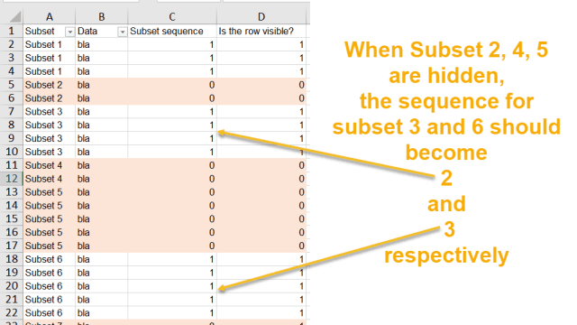
When rows are hidden by filter, the corresponding values in column D will become 0.

When this happens, we want

1. to reset the Subset sequence for Subset 2, i.e. values in C5:C6 from 2 to 0
2. to change the Subset sequence for Subset 3, i.e. values in C7:C10 from 3 to 2 (this is the most tricky and challenging part)

Challenge 2.1 – Reset the subset sequence for hidden rows

We can solve this by multiplying C2 with D2

In C2, input the formula:

=IF(A1=A2,C1,SUM(C1,1))*D2   ‘copy down

=

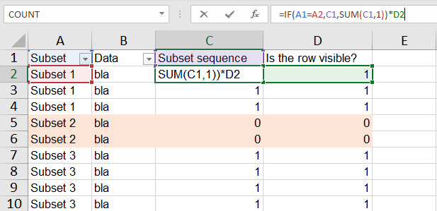
So now, when a subset is filtered out, the subset sequence becomes 0.  The rows will also been highlighted if we used ISEVEN for the conditional formatting… but it doesn’t really matter as we won’t see it (when it is hidden). 😛

Challenge 2.2 – Adjust the subset sequence for the next visible group

Let’s exam what the original formula does.

=IF(A1=A2,C1,SUM(C1,1))

The blue portion of the formula SUM(C1,1) tells Excel to add 1 to the number above the current cell when it detects a change in “Subset” (when A1=A2 is False).  It works fine when we do not filter the data.

However, when a filter is applied, the formula doesn’t work properly.  It returns 1 to all subsets that are next to the hidden subsets, because the sequence for hidden subset is reset to 0.

To achieve this, we need to twist the blue portion of the formula

from

=SUM(C1,1)

to

=SUM(MAX($C$1:$C1),1) ‘Note the usage of $

By using =SUM(MAX($C$1:$C1),1), we instruct Excel to add 1 to the maximum number above the current cell.  It looks through from the very first cell on the top to the cell that is just above the current cell.  As such, the 0 resulted from hidden rows is ignored.

And we will get the correct sequence after filtering. 🙂

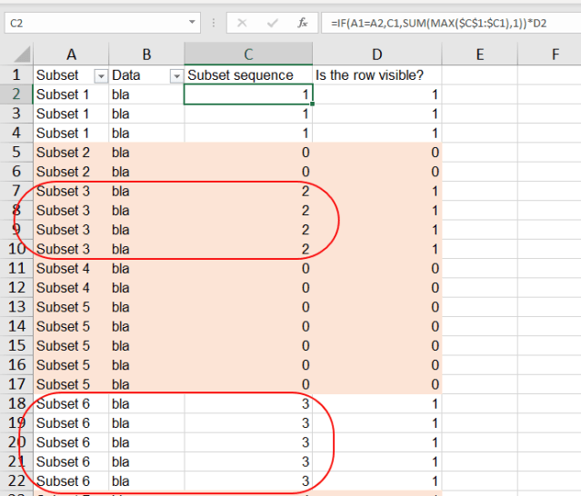
Challenge 2.2 is solved with this formula:

=IF(A1=A2,C1,SUM(MAX($C$1:$C1),1))*D2

Tip: You may substitute SUBTOTAL formula in D2 into the formula, i.e.

=IF(A1=A2,C1,SUM(MAX($C$1:$C1),1))*SUBTOTAL(103,A2)

so that you won’t need the extra helper column for identifying if a row is visible

Wrap up

Putting everything together, we need the following formula for the helper column:

=IF(A1=A2,C1,SUM(MAX($C$1:$C1),1))*SUBTOTAL(103,A2)

Then we apply conditional formatting to the range A2:C29 by the following formula:

=ISEVEN($C2)

Make sense?

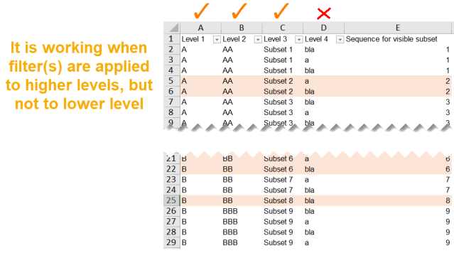
Limitation

Indeed this solution is not working in all scenarios.  If you have multiple levels of hierarchical data, it works well only when you reference to the lowest level of data.

If you set the formula in helper column based on value on column C, but you apply filter to Column D, you may break the conditional format.

Try it out with the Sample File.

Thanks Casey for the question.  I hope this solves your problem.  If it does, please share this. 🙂