When setting up conditions for Conditional Formatting in Excel, have you ever tried to set a formula that refers to a Excel Table, but failed?
First of all, why we want to refer to Excel Table in Conditional Formatting? There is one simple answer: To accept new data automatically.
Let’s look back at the sample we used in the previous two blog posts. In the following screen shot, you see that the formula used refers to a “fixed” range of $I$2:$I$9. It works totally fine given the current static situation. 
But what if we are moving into May and are ready to input more “PublicHolidays” to the list?
Oh no… it didn’t work as the formula was hard-coded.
To fix that, we need to go into the formula of Conditional Formatting and revised the hard-coded range. (provided that you remember to do it; and/or your user knows how to do it) 🙂

That’s why we want to make the formula used in Conditional Formatting be dynamic!
There are two common ways to do dynamic ranges:
- Using OFFSET function
- Using Excel Table
Using Excel Table will be the technique discussed in this post. Indeed, whenever possible, I highly recommend you use Excel Table for dynamic range. Excel Table was introduced in Excel 2007. After a decade, it’s still one of the hidden gems to most regular Excel users. We should promote it more as it is really a cool feature of Excel. Indeed there are obvious reasons of using Excel Table over OFFSET for setting up dynamic range. Nevertheless that is not the topic of this post. 😛
To turn a range into Excel Table
- Select the range
- Go to Insert tab
- Click Table
- Check the range is correctly detected; and My table has headers is checked
- OK
Tip: Keyboard shortcut for inserting a Table: Ctrl+T
As a good practice, always name your Excel Table to something meaningful to you/users. In our example, it’s named as tb_PH.
Now, we have created an Excel Table named tb_PH. Let’s try two things:
First, let’s see what happens when
- we select tb_PH from Name Box; and
- after new data is added to tb_PH, repeat step 1 and see
wow…. tb_PH accepts new data appended. Now the same table name tb_PH refers to an expanded range. Isn’t it cool?
Now, try also this:
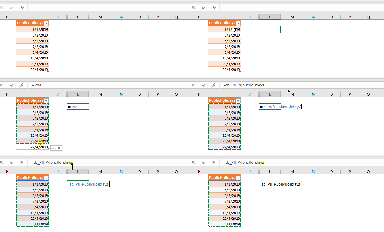
In any blank cell, input = then using mouse to select the range I2:I9
Note: For demonstration purpose, the range before adding data is used. If you have added new data to tb_PH, ensure you have selected the whole range to make Excel to turn the range into a Structure Reference automatically.
See?! Excel automatically turns the range selected into a Structured Reference:
=tb_PH[PublicHolidays]
Don’t be afraid of the new formula structure. It simply refers to the Table Name [ColumnHeader]. In other words, it means the (whole) column of PublicHolidays of the table tb_PH.
On the surface, you may know what I am trying to do next – Using the Structure Reference in the formula for conditional formatting:
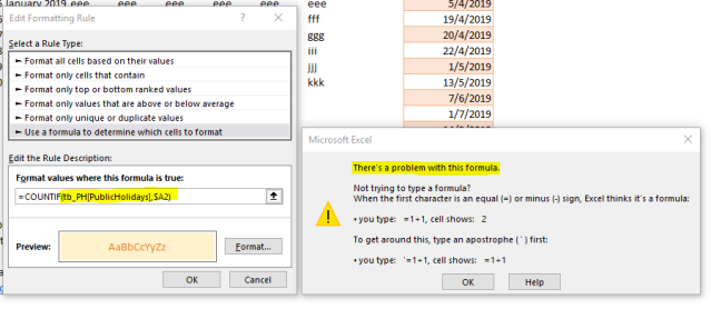
=COUNTIF(tb_PH[PublicHolidays],$A2)
Unfortunately, it did not work….
To test the formula, copy it and paste it to K2 and see:
It works. Somehow it does not work in conditional formatting…
To fix this, we need an INDIRECT approach in the formula set:
=COUNTIF(INDIRECT("tb_PH[PublicHolidays]"),$A2)
And the trick is… simply wrap the Structured Reference with INDIRECT. (Note: Don’t miss the double quotes)
As simple as this. 🙂
Let’s watch the result in action:
WOW… it works like a charm! 🙂
Tip: As there is only one column in the Excel Table, we may shorten the formula to:
=COUNTIF(INDIRECT("tb_PH"),$A2)
Want to know about what COUNTIF does in the example? Please read the post Highlight weekends and holidays using Conditional Formatting in #Excel.
You may download a sample file to follow along. Remind you to unhide the sheet <Example (3)>.


You are welcome 😄
LikeLike
You are awesome
LikeLike
My biggest issue is not the formula per se, but the range “Applies to”. If there’s a change in the table (e.g. adding a row/collumn in the middle) this messes up the range… THERE I would also like to use a structured reference (that hopefully wouldn’t change, if the row/column order changes).
LikeLike
Structured reference in Excel table is an awesome feature 👍🏻
LikeLike
Thanks for your detailed suggestion. You are right about INDIRECT. We should avoid use it massively. Nevertheless it should be fine for small size workbook. 😁
LikeLike
I have one issue with this approach: INDIRECT is an inefficient function, and should be a last-option to refer to. It’s a Function after-all, meant to interpret a value.
A better solution is to use:
1) A table, for convenience. For example, we’ll create a table with [ID], [first name], [last name] with the table-name [clients]
2) Create a “Named array” from the contents of this table, without the header
(it can be a sub-selection of the table, like [ID]:[Last name])
2a) Make a selection of the contents of the table
2b) Go to: Formulas > Name Manager > New…
2c) Give a name, I usually take the name of the table with an underscore in front of it: [_clients]
Scope: Workbook
Give a declarative comment if you want
Check if the Referens is correct:
=clients for the contents of the whole table
=clients[[ID]:[Last name]] if you want just a range within the table (useful for large tables and saving some time)
3) Now you can refer to an exact range of values with your conditional formatting. This is a lot faster then a computational function And you can do things like
=VLOOKUP($A2;_client;3;FALSE)=”Anderson”
Or in your case:
=COUNTIF(_tb_PH,$A2)
AND keep the flexibility of tables. 🙂
LikeLike
@Bl4derubber …
The topic was referring to the use of “Structured tables” in Excel. Your response included the use of “Name Manager” and “VLOOKUP” function. As soon as I see that, I realized you are not familiar with structured tables in Excel so I don’t bother reading the rest of your message.
Research Structured tables in Excel … It’s an awesome hidden gem in Excel since 2007, and I have worked with those that consider themselves as “experts” in Excel, but are totally unaware of the structured table capabilities in EXCEL.
LikeLike
This approach works perfectly, with structured tables, in a way that the INDIRECT approach did not for me.
I have two tables on two different tabs. I use a Named Range (named array) from Table 2 to create a data validation list of values to be used in Table 1. I want the cells in Table 1 to turn red if the value is no longer part of the valid list of values. The most direct way to accomplish this would be to use a XLOOKUP or VLOOKUP nested in a ISNA function, using table references in the lookup. However, the conditional formatting does not support the table references. By creating a named range (lstPages) for the target list (Table 2[Page List]) I am able to use the following formula in the conditional formatting:
=ISNA(XLOOKUP(G3,lstPages,lstPages))
In addition, I am able to use the same named range as the source for the Data Validation in Table 1.
Perfect suggestion @Bl4derubber, thank you.
LikeLike
I believe you’ll also find that simply writing your conditional formula to refer to an entire column from a Table somehow enables that range reference to auto-magically grow as the Table grows without needing to use INDIRECT or other trickery. In fact, if your cursor is on a cell of that Table when you bring up the Conditional Formatting Rules Manager, then the dropdown to “Show formatting rules for:” will contain an option for “This Table” in the pick list.
LikeLike
That’s brilliant! Thanks for sharing David. I will show it on next post.
LikeLike