…When the layout is bad…

Here’s the situation:

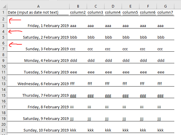
1. There are blank rows between each rows with data;
2. We want to highlight both rows (the blank row and the row below when that’s a weekend), i.e. Row 4, 5; 6, 7; 18,19; 20,21) in the above example.

Well, you may not consider the above layout bad.  Indeed it is quite common in workplace.  A blank row is inserted for whatever reasons (and some people quite insist on it)…

Let’s see how this “bad” layout complicates the whole process of setting up of conditional formatting to highlight weekends.

Note: This post is a continuation of previous post.  You may want to read the previous post first if you do not know how to use conditional formatting to highlight weekends.

Instead of setting up one formula in one range of data (as what we demonstrated in previous post), we need to create two conditions for multiple ranges.  Before we jump into multiple ranges, let’s focus a smaller range, say A2:G3.

• For the blank row (A2:G2), we need to look into the first cell one row below (A3).  If that cell is a weekend, then highlight the current blank row (A2:G2);
• For the row with data (A3:G3), we need to look into the first cell on the same row (A3).  If that cell is a weekend, then highlight the current row (A3:G3).

So this is what we gonna to set up with conditional formatting:

Note that there are two conditions with one common formula:

=OR(TEXT($A3,"DDD")="Sat",TEXT($A3,"DDD")="Sun") 'Applies to $A$2:$G$2
Note: Pay attention to the row we used in the formula; and the row the formula applies to.
There is one row offset.

=OR(TEXT($A3,"DDD")="Sat",TEXT($A3,"DDD")="Sun") 'Appleis to $A$3:$G$3

By now, you may be thinking… why we need to apply the same formula to two different ranges?

Let’s see what if we don’t:

In the above screencast, we apply the formula to a continuous range of $A$2:$G$11 and we’d got the following result:

Obviously this is incorrect.

You see that all rows with data is highlighted; while two blanks rows are highlighted correctly (the row below is weekend).

But why?

To find out why, we need to understand

1. What the formula set to the ranges do?
2. What is the value return by a formula that refers to an empty cell?

1) Let’s examine the formula used and the range it applies to:

Formula: =OR(TEXT($A3,"DDD")="Sat",TEXT($A3,"DDD")="Sun")
Applies to:
=$A$2:$G$11 

Note the difference in the row reference.  Put it into words, in the range of $A$2:$G$11, Excel refers to the first cell one row below and see if it is a weekend.  If it is a weekend, highlight the current row of A:G; do nothing if it is not a weekend.

2) What is the value return by a formula that refers to an empty cell?

The answer: 0 (zero).  But why Excel considers 0 as weekend?

Did you know…the first date recognized by Excel (for Windows users) is 1/1/1900, which is stored as a value of 1.  And coincidentally 1/1/1900 was a Sunday, making the “imaginary” 0/1/1900 a Saturday.  In short, if we ask Excel to evaluate the day of an empty cell, Excel answers: “It is Saturday”.

Got it?

Now let’s examine 1) and 2) together row by row:

On Row 2 (A2:G2), the condition is set to examine the value in A3 to see if it is a weekend.  Well it is not, that’s why Row 2 (A2:G2) is not highlighted.

On Row 3 (A3:G3), the condition is set to examine the value in A4 to see if it is a weekend.  Well it is a blank cell, it means 0 to Excel which happens to be “Sat”, that’s why Row 3 (A3:G3) is highlighted (incorrectly).

On Row 4 (A4:G4), it looks into A5 to see if it is a weekend.  Well it is, that’s why Row 4 (A4:G4) is highlighted.

On Row 5 (A5:G5), it looks into A6 to see if it is a weekend.  Well it is a blank cell, it means 0 to Excel which happens to be “Sat”, Row 5 (A5:G5) is highlighted (incorrectly).

And so on and so forth…

This is the reason we cannot simply apply one formula to one continuous range, thanks so much to the empty row inserted.

Well, we have the problem, then what’s the solution?

Because we are working with Excel, we have more than one approach to solve a problem. 🙂

Approach 1 – Applying the two formula to multiple ranges

As explain before, we used one formula for two different range to set the conditional formatting right.  We can now extend the “Applied to” range to multiple corresponding ranges, like the screencast below:

Although it’s doable, it’s not recommended.  Think about the time and the concentration required, especially when you are dealing with more rows.  Think about to do it for a month of data… Do you want to use this approach?  I don’t.

Approach 2 – Using a helper cell and then make it invisible

First to select all blank cells above “dates”

1. Select the range, A2:A21 in our example
2. Ctrl+G to open the “Go To” dialog box
3. Special…
4. Select Blanks
5. OK

Second, input a formula to make the empty cells equal to the date below

When all the blank cells are selected, input

=A3

then Press Ctrl+Enter.  This action inputs the same formula to all selected cells.

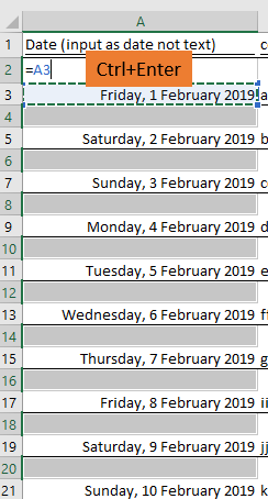
Note: Make sure the active cell is at A2 when you input the formula =A3

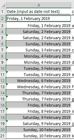
Now you should see all the empty cell on top of the date is filled with the same date below.

Third, make these helper cells invisible, simply format them (Press Ctrl+1 or Right-Click)

1. Select the “Number” tab
2. Select “Custom”
3. Input three semicolons ;;; in Types
4. OK

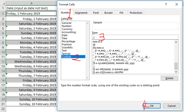
This is a useful trick to make cell contents invisible.

Forth, set up the conditional format in the easy way

1. Select the range A2:G21
2. Go to Home –> Conditional Formatting –> New Rule…

This is the formula applies to the range A2:G21

=OR(TEXT($A2,"DDD")="Sat",TEXT($A2,"DDD")="Sun")

Here we go! 🙂

Indeed this is a good example to demonstrate again how a “good” layout (without blanks) makes the set up easier.

Well… for whatever reasons you cannot input anything on the empty cells above dates because the cells are left blank intentionally for users to input remark…

Ok… I heard that.  Approach 3 comes to rescue.

Approach 3 – Setting two conditions to two continuous ranges

The core of the two conditions has been discussed in Approach 1.  Yessss… these are the two conditions:

• First, the formula looks into one row below;
• Second, the formula looks into current row.

However, we need to modify the two formula a bit to adapt to the “empty” row problem that returns 0, which misleads Excel to consider it “Sat”.

To format empty rows

As discussed in Approach 1, applying a formula to multiple ranges may not be ideal.  So we try to apply one formula to a continuous range, which is A2:G20 in our example.

Let see again what happens if we do not modify the formula:

Formula: =OR(TEXT($A3,"DDD")="Sat",TEXT($A3,"DDD")="Sun")

Applies to: $A$2:$G$20 
'Note: The range is up to the second last row of the data set.

Oooops… all rows with data are highlighted because Excel evaluate empty cells one row below.  As discussed, Excel considers empty cell as “Sat”.  That’s why all rows above empty rows are highlighted.  To avoid this, we need to modify the formula to consider if the first cell on the row below is empty or not.

And the modification is simple:

=OR(TEXT($A3,"DDD")="Sat",TEXT($A3,"DDD")="Sun") * ($A3<>"")
Applied to $A$2:$G$20

Yes.  It works.

Why it works?

The portion *($A3<>””) evaluates if the first cell on the row below contains value or not.  The operator * essentially sets an AND condition.  In plain English, if the first cell on the row below is not blank AND it is either Saturday or Sunday, then highlight the current row.

Want to learn more about using * and + in setting up logical tests, read this post.

To format rows with data

Using the same formula, but applying to a different range $A$3:$G$21 (one row offset), we can set up the conditional formatting correctly.

To summarize, we solve the problem by applying one formula:

=OR(TEXT($A3,"DDD")="
Sat",TEXT($A3,"DDD")="Sun") * ($A3<>"")

to two different ranges:

$A$2:$G$20 'which evaluates row below
$A$3:$G$21 'which evaluates current row

As simple as that. 🙂

You may download a sample file to follow along.  I did not demonstrate how to highlight public holidays in this post on purpose.  That’s your homework.  Let’s see if you have grasped the concept well.

When there is obstacles, there will be workarounds (most of the time).