How to insert thousands of rows for each change in item in a column?  And then give a subtotal of each item?

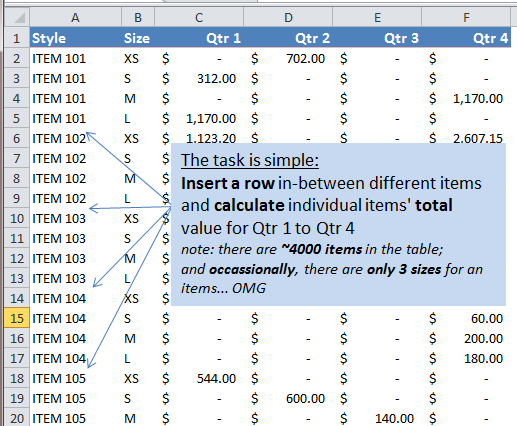
Long long time ago (>10years) when I was only an Excel newbie, a friend asked for help.  She was desperate for the task given.  She had no clues and planned to do that manually.  You can imagine how long it would take – FOREVER.

I spent a while, maybe an hour, to record and test some Marcos for the repeating “Copy and Insert Copied Cells” actions. Finally I solved her problem in much less time than she expected.  And we were so happy the problem was solved.  The luck we had was there were always four rows for an item.  If it happened to have irregular number of rows for different items, like in our example, I am sure that I won’t able to solve her problem, at that time.

Today, I know that this kind of problem can be solved in less than a minute WITHOUT any hassle.  Thanks to Data->Subtotal

Let’s do it step by step

1)     Select the Data Range (although it is not necessary as Excel is smart enough to guess the range, I would still recommend you to do so as there are chances for incorrect guessing)

2)     Go to Data -> Subtotal to open the Subtotal dialogue box

3)     Select appropriate items accordingly, as shown below:

As we want the subtotal to be inserted for different ITEM, we select “Style” which is the header for different ITEMs

• Use Function: Sum. You may choose from all the available functions for SUBTOTAL
• In the “Add subtotal to:”, check all that you need.  In our example, they are Qtr 1, 2, 3, 4
• Check / Uncheck the bottom three options per your need
• OK

Well, I know that. You expect Excel to give you result at a blink.  But the truth is we are dealing with 16000 Rows and inserting more than 4000 rows of subtotals.

After 35 seconds…

Here we go:

See! Not only does Excel insert rows of subtotal for all different items, it also groups the items.

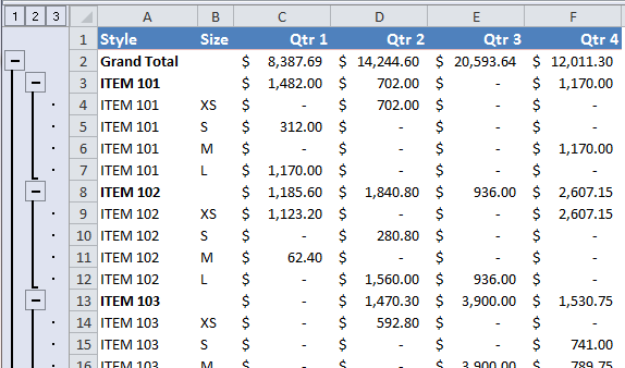
Let’s click on “2” just below the Name Box.  The grouping offers you to see the subtotals only.

By clicking on a “+” , you can see the details for the grouped data.

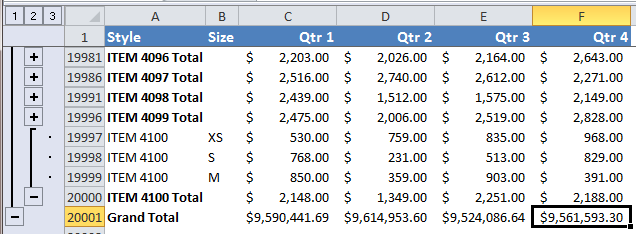
Regardless number of rows for an item, Data->Subtotal manages identify each change and apply Subtotal at each change.

Tips:

• This is how the result looks like if you uncheck “Summary Below Data” in step 3

• The column(s) of interest (in our example: “Style”) must be sorted (ascending or descending doesn’t matter) in order to group data for same item together

Just in case you need to remove all subtotals: Go to Data -> Subtotal -> Remove all