Part 2 – What if we have inconsistent table structures across files?

Note: this is a long post. 😉

This is the continuation of previous post. Suggest you read that post first if you are new to Power Query. Moreover you may download sample data files there to follow along.

In the previous post, we used Power Query to combine all files in a folder. With that built, we can get new data file by a simple click of Refresh. The following screencast shows you that we have combined three data files. When a new file – Week 4 data, comes into the folder, we can easily get the new data by a click of Refresh.

Watch this:

Before Week 4 data, there were 63 rows of data. After we have 84 rows of data.

Isn’t it great? It is awesome! 😎

Then next week, we have data file for Week 5. We feel great as we expect a consolidated table by putting the data file into the same folder, followed by a click of Refresh… BUT…

we didn’t see the date of week 5, but (Blank)? What happened? 😨

Let’s have a closer look at the Queries & Connections Pane

You can download the data file and working file to follow along.

After the query refreshed, with the data file of Week 5 put into the folder, there were 106 rows loaded and 1 error. Wait… before we had 84 rows, now we have 106 rows. Does it mean we have the new data combined?

Not really. Let’s look at the table loaded on worksheet… scroll all the way down:

We have a blank row + many rows of data with nothing on column A to C.

1 error?

Clicking on “1 error” will take us to an auto-generated query that shows what happened, kind of…

1. The query that is created by Power Query automatically
2. The error happens on row 85
3. Click the cell of “Error” (not on the word “Error”; but empty space in the cell), it shows what happened: Power Query could not convert “HKD” to Number.

At this point, it is not yet crystal clear but we have clues to explore.

When we go back to the “CombinedTable” query, we see that there is an error on row 85, which is the result from the unexpected data “HKD” because Power Query fails to convert it to a number. However we have no idea why all subsequent rows contains “Sales Amt” but nothing for “Site ID”, “Date”, and “Sales Qty”.

Let’s go back by three steps to “Invoke Custom Function“

Since we encountered this problem when week 5 data came in, we can focus on comparing the tables extracted from the 4th and the 5th files.

Now it is clear that the headers in Week 5 data are not the same as previous table.

Still remember how the Week 5 data look like?

It looks like this:

Row 1 contains “Blank”, “Blank”, “Blank” and “Sales Amt”.

And do you remember what transformation step we did in the sample query?

Bingo! We promoted first row as headers.

When first row of week 5 data is promoted to headers, we get the following:

The first header is “blank”, the second and third header is also “blank”. As Power Query does not accept duplicated headers in table, it adds a numbered suffices to those duplicated headers. That’s why we have “_1” and “_2” as the column headers. The final column “Sales Amt” is correctly promoted as header.

Now going back to the “CombinedTable” query

Let’s try to locate the step that leads to the error, by walking through the steps one by one.

No error detected so far up to here.

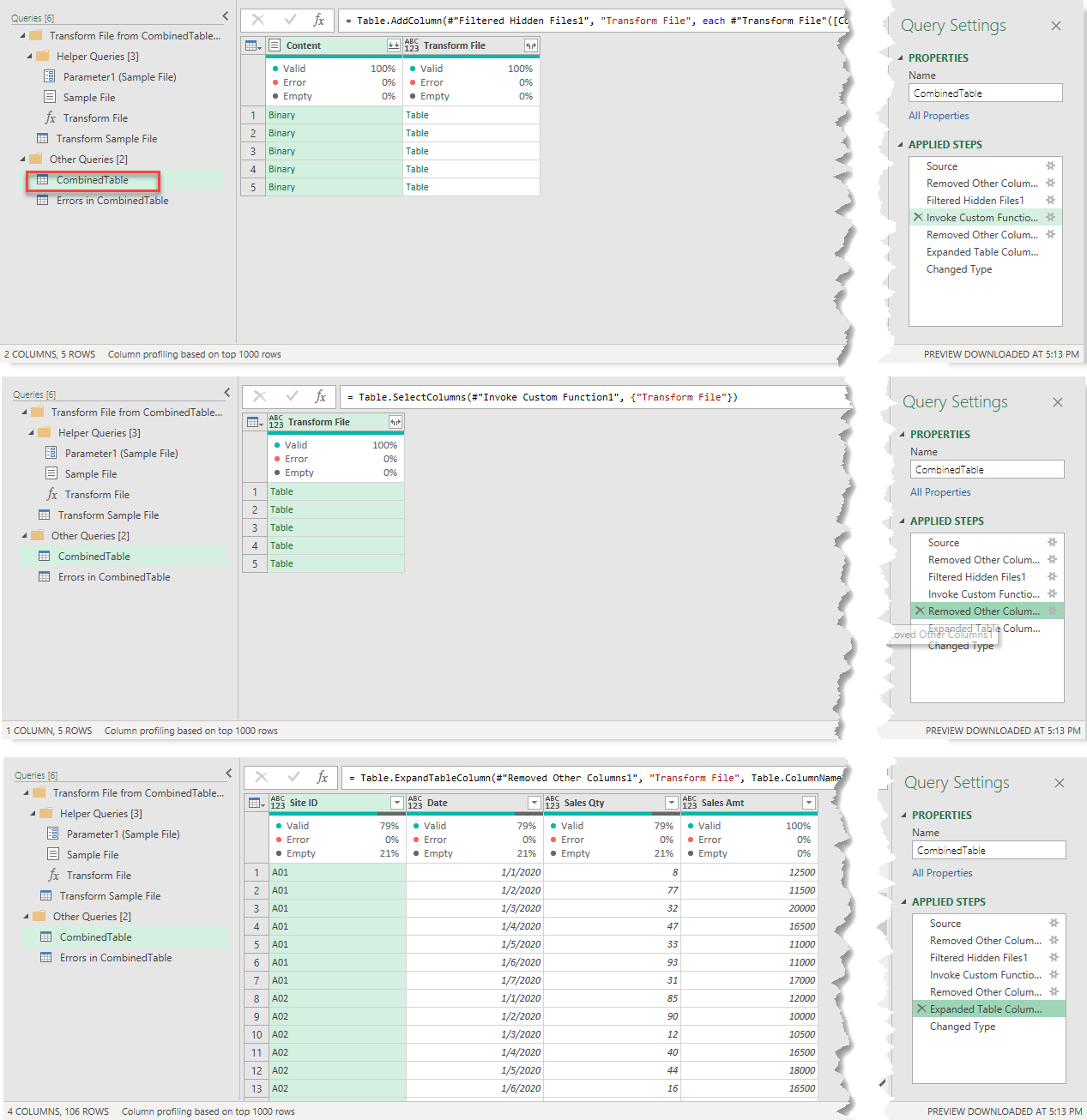
Before we move to the last step “Changed Type“, I would like to draw your attention to the step “Expanded Table Columns1” which is the step Power Query appends tables together into one single table.

When Power Query appends tables, it looks for common headers to append the data. Since we have a layout change in Week 5 data, we do not have consistent column headers across different tables. As shown on screenshot below, the only common header found in Table 5 (week 5 data) is “Sales Amt”. As a result, all data under “Sales Amt” including the word “HKD” will be appended to the final table.

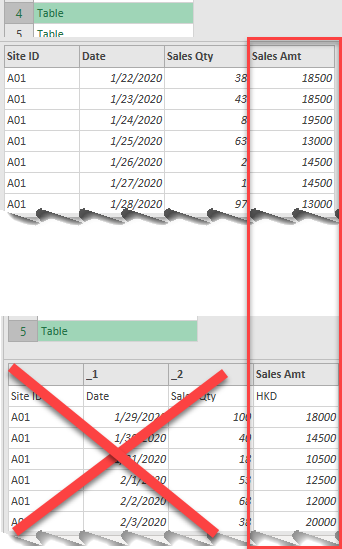
The first three columns in Table 5 are ignored. To be more precise, the four columns “Site ID”, “Date”, “Sales Qty” and “Sales Amt” on the sample file are being used (hard-coded) in the step for “Expanded Table Columns1“. Any columns else that may appear in other files are therefore ignored.

We can confirm this behavior if we move on to the step “Expanded Table Columns1” and scroll down to row 85, where the first row from Table 5 is.

Note: I have a blogpost for more details about appending tables.

The final transformation step “Changed Type” results in the “Error” as Power Query cannot convert “HKD” into a number. This makes sense.

In summary, the query for combining tables in a folder are broken due to the slight change in column headers in a data file. The query still runs, but it does not give the result expected.

When we understand the problem. We can (probably) fix the problem.

As a rule of thumb, if you need to transform (or reshape) your data for combining files, do it in the “Transform Sample File” query.

From previous post.

This is also where we go for debugging most of the time. 😁

Before you tap into a solution, let’s set the goal here:

Make a sample query that cleanse both table layouts

To start with, we go back to the sample query “Transform Sample File“.

Nevertheless, the sample file selected is already in a good shape. It would be easier to work on the problematic file, i.e. Week 5 data. So we go to the Sample File…

1. Select “Sample File“
2. Select the first step “Source“
3. Click the “Refresh Preview” to reveal the newly added data files

Then we may select whatever file we want as the sample file.

In this case, we want “Sales_Wk05.xlsx” to be the Sample File.

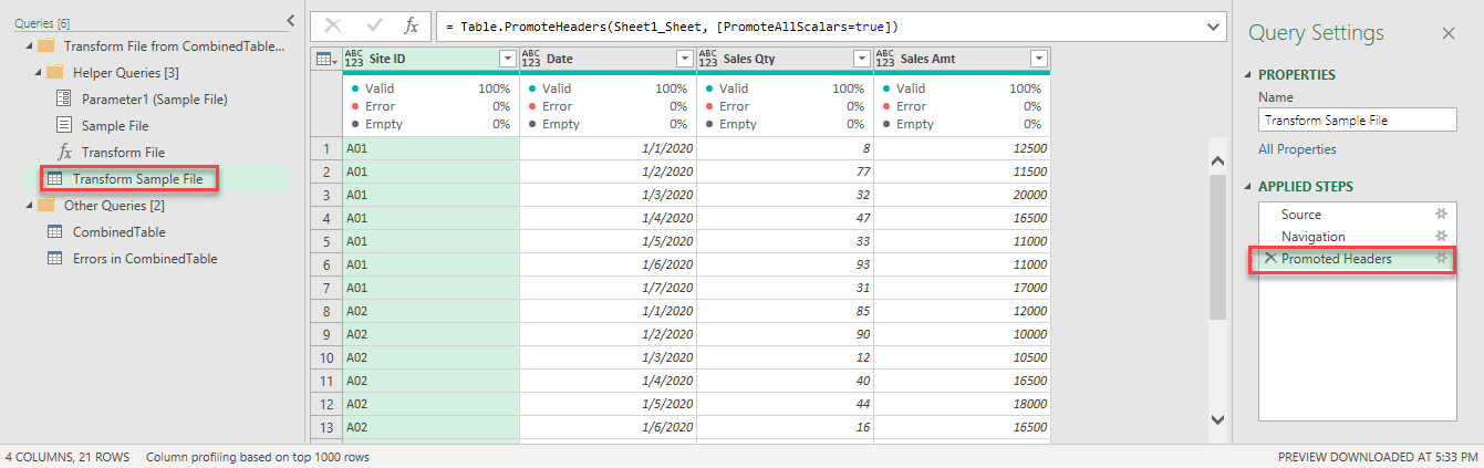
Now going back to the “Transform Sample File“. We see it’s updated using Week 5 data as sample: Only “Sales Amt” is correctly promoted; while Column1, Column2 and Column3 are being used as the column headers because “blanks” are promoted.

We definitely do not want Column1,2,3 as the headers. As we checked with I.T. (pls refer to previous post for the story) that the order of the columns will not change, we feel comfortable to change the column headers directly by doubling clicking the headers, one by one.

In order words, we want to rename the column headers manually. To ensure we have consistent column headers before renaming, we need to remove the step “Promoted Headers“.

Now we have Column1,2,3,4 regardless of the data file we pick.

Then we can rename Column1,2,3,4 to “Site ID”, “Date”, “Sales Qty”, and “Sales Amt” respectively.

Now we are very tempted to use the “Remove Top Rows” to get rid of the first two rows of data that is no longer required…

DO NOT DO THIS!

Remember: Our goal is to create a sample query that cleanse both table layouts. If we set up a step to remove top two rows here, this step will be applied to all tables. In short, this dangerous step removes the first (valid) data record from all previous data file. This will lead to a mistake that is hard to be discovered on big dataset.

So how to get rid of the first two rows from Week 5 data onwards without damaging the data integrity of previous data file?

Easy, we can “Filter out” the rows that we do not want:

When this step is applied to tables where there is only row of headers, no row with valid data will be removed. Make sense?

From now on, when week 6 data comes, we will have the magical click of Refresh back to work, in the way we expected. 😎

You may download a sample workbook with the modified queries below:

Final note

There are more than one way to fix this problem. In real life, the difference in table layouts could be more complicated. The solution suggested here will never be an one-fit-all solution. The idea is to pinpoint how we could locate the steps that lead to problem; and try to find a way to fix it. Most of the time, the thinking process is even more important than the solution itself, I believe…

Hope you like it. 😉