Can you spot the error in the above formula?

It’s not about the new function of XLOOKUP.  It’s about inevitable human error…

If you are an Excel fan, you should be aware of the exciting XLOOKUP function in Office 365.  It is, no doubt,  an awesome function that will beat VLOOKUP, HLOOKUP, LOOKUP, INDEX/MATCH in the future when it is generally available to all Excel users.  You may find more details about XLOOKUP from Microsoft Tech Community.

There are many very well presented videos about XLOOKUP on YouTube already.  Just to name a few (my favorite YouTube channels),

• Leila Gharani
• ExcelIsFun
• Excel on Fire
• MrExcel 

So in this post, I am not going to talk about all the cool features of XLOOKUP.  Instead, I would like to draw your attention to a potential mistake when writing XLOOKUP function.

You may download a Sample File to follow along.

Now let’s look back to the question:  What’s wrong with XLOOKUP? 🤔

A major difference between VLOOKUP and  XLOOKUP is how they handle the return array.

In VLOOKUP, we need to identify the table_array as the 2nd argument, and specify the column to be returned, as the 3rd argument.  Because of this, VLOOKUP searches from left to right, which is exactly one of its well-known limitations.

In the new XLOOKUP function, the lookup_array and the return_array are now two separate arguments:

Thanks to this improvement, XLOOKUP is highly flexible!  XLOOKUP can lookup vertically, or horizontally, regardless of lookup directions.  Nevertheless, it opens a door for potential human error.

What is that potential error?

A picture tells thousand words:

In this example, the formula input in E2 is

=XLOOKUP(D2,A2:A11,B3:B12)

With the visual aid above, and given the small data range for the purpose of demonstration, we may spot the error quickly.  BUT when we are dealing with a large range of data, this kind of “careless” mistake could be a fatal spreadsheet error as it’s not easily spotted.

Luckily, Excel is care enough to give us a warning sign for such case.

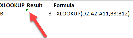
Do you see that tiny green triangle?

It means that there may be something wrong in the cell.  Let’s take a further look at the message by selecting the cell, followed by clicking on the “Exclamation mark” next to it.

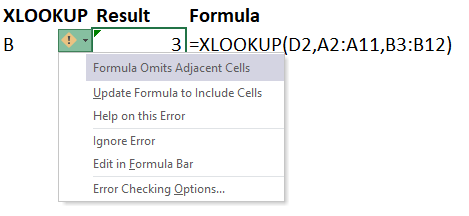
It says: “Formula Omits Adjacent Cells” and it offers a suggestion: “Update Formula to Include Cells” to fix the issue.

Let’s try and see:

Oops… it returns #VALUE error.

Why is that? Because…

Here’s the revised formula:

=XLOOKUP(D2,A2:A11,B2:B12)

Excel revised the return_array from B3:B12 to B2:B12.

When the lookup_array and the return_array are of different sizes, XLOOKUP returns #VALUE error.

Although Excel is not intelligent enough yet to fix this mistake correctly, it successfully draws our attention to have a closer look at the formula; and hence has a higher chance to fix it manually by ourselves.

By the way, did you ever pay attention to that tiny green triangle? Be honest 😁

Next question in my mind

What about approximate match?

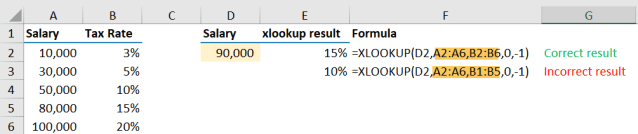
Well, it behaves the same as exact match.  It returns a “shifted” result; depending on the range offset between the lookup_array and return_array.

Interestingly, the tiny green triangle does not appear in this case.

By now, if you have followed through, the question should be

WHY IS THAT?

I think it is not uncommon for you to expect XLOOKUP works the way you think, even though there is a shift in the return_array:

Hey, Excel… Did you see… 2 is in a parallel position to B.

How come you return 3 instead? It doesn’t make sense…

It never happened in VLOOKUP.

Well, I believe it is due to the same issue I discussed in my another post Be cautious when using SUMIF(s).  It is about the position of the matched value in the ranges.  Please read that post for details.

How to avoid this?

Now we know there is an issue, is there a way to avoid it?

I said many times in this blog:

If human error can be avoided, it’s not human error at all. 😛

Having said that, I strongly suggest we use Structured Reference with Excel Table.

This is an easy but highly effective way to avoid careless mistake we discussed so far.

In short, to make XLOOKUP work in the way you think, you need to ensure two things:

1. lookup_array and return_array must be of equal size
2. lookup_array and return_array must be aligned perfectly in parallel

Why Excel has this kind of bug in such a powerful new function?

Well, I won’t say it’s a bug.  It should be a feature, I guess. 🙂

In rare cases, you may want Excel to perform a VLOOKUP but return the value that is at the next row of the match.

Consider a table layout like this:

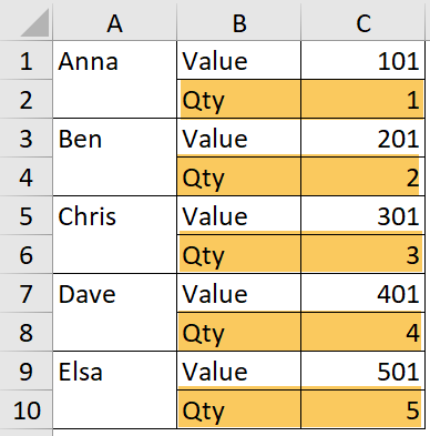
What you want is to lookup the Qty by Salesperson.  In this case, the traditional VLOOKUP would not work.  INDEX/MATCH comes to recuse.  But now, if you have XLOOKUP, you may consider using it to solve this scenario too! 😉

Watch this:

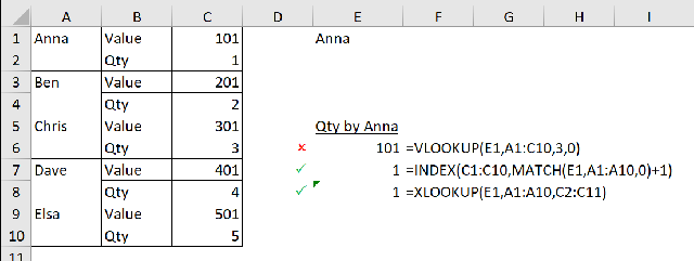
Just pay attention to the shift in the return_array you need.  That said, it may not be an efficient formula when you want to return “Value”, or even better to make “Value” and “Qty” a parameter for user to select from.  INDEX/MATCH would be a better choice then.

That’s it.

Do you have other practical use case of XLOOKUP where you would like to return a shifted value in the return_array?  If you do, please share with us by leaving comment below.

You are more than welcome to share your use cases of XLOOKUP too. 😉