The recent HOT topics about Excel should be the new Dynamic Arrays! After watching all the amazing demonstrations about the new Dynamic Arrays, I’ve decided to sign up to the Office Insider (Fast) programme (for Office 365 subscriber only). And I finally got it last Saturday. I was thrilled to try it out. Simply awesome!
Then I try to solve a problem with the new dynamic arrays – Creating a shrinking dropdown list, as shown below.

It is a common task to assign people to different groups. Once a person is assigned to a group, s/he should not be shown up again from the dropdown list in order to avoid duplication.
In “old” Excel, I needed three helper columns, with a “scary” array-formula, together with the old-school trick to create a dynamic list by using OFFSET function as Named Formula. It took me quite a while (in terms of hour) to figure it out and make it work correctly.
With the new Dynamic Arrays in Excel 365, I need only one helper column with simple MATCH function + Dynamic Array. And believe it or not, it took me only a couple of minutes. Let’s see how:
You may download a Sample File to follow along IF you are on Excel 365 Insider Program.
Set up the Tables
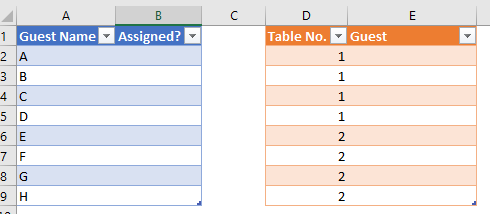
Create two Excel Tables, as shown below:
- GuestList (where we have a list of people)
- AssignTable (where we put the dynamic list)
Note: To convert a range into Excel Table, select the range –> Ctrl+T or Insert, Table

Tip: As a good practice, always name your Table with a meaningful name:

Set up the formula in helper column B
In B2, input the following formula:
=MATCH([@[Guest Name]],AssignTable[Guest],0)
Don’t be afraid of the Structural Reference used in Table. You may input the MATCH formula by using a mouse as if writing a normal formula, Excel will do the conversion for you. Watch the following:

Now try to input a Guest Name, say B, in E2.

Technically, when a guest is assigned to the Table “AssignTable”, it returns a value; otherwise, it returns “#N/A”. This is what the formula just input does. Now we have the basis for filtering a list of non-assigned guests.
Set up the Dynamic Array formula
In H2, input the following:
=SORT(FILTER(NameList[Guest Name],ISNA(NameList[Assigned?]),"All Assinged. Good Job!"))
Note: I am not going to go through the new functions in details, which is not the intention of this post. If you want to learn more about the new functions, I highly recommend you watch the YouTube videos from ExcelisFun and MrExcel.com. You can find the links to the videos in my post – Exciting Dynamic Array functions in #Excel 365.
Let’s see it in action:

wow… Did you see it? A list of “non-assigned” guest was generated.
What’s more interesting & exciting, the list changes dynamically with the input in the [Guest] column:

Pay attention to the changes in Column H with the input.
Set up the Data Validation
Now, you probably know what comes next. Nevertheless, you won’t believe how easy it becomes:
- Select the [Guest] column
- Go to Data Tab
- Data Validation…

In the Settings of Data Validation, select “List” and then input the following formula in Source:
=$H$2#

Important: The key is the hashtag # that tells Excel it is a dynamic array originated in H2. Note: Absolute row is required here.
Now, watch everything in action. Pay attention to the changes in the column [Assigned] and the Dynamic Array returned at H2, with the input.
Simply awesome. Isn’t it?
Unexpected error:

As you know, we can input the cell with data validation either from the dropdown menu or directly input (as long as the input is valid). However, I got the above error when I tried to input a name manually.
Watch this:

So weird! Then I further experimented on UNIQUE and FILTER functions and fed the resulting arrays into Data Validation, they all worked normally as expect – I could either input the cell from the dropdown or manually.
One step further, I used RANDBETWEEN in a small dataset. The resulting dynamic array from FILTER function changes whenever I input something. Interestingly, the data validation accepted input from the dropdown always. Nevertheless, it worked occasionally (indeed randomly) for manual input.

Apparently, inputting a cell manually trigger a recalculation before the cell content being sent to the validation process. It makes sense to me because RANDBETWEEN is a volatile function. Because of this, there are chances that the “re-calculated” array does not carry the label we input and hence the data validation rejects the input. Interestingly, inputting the cell by dropdown menu trigger the recalculation after the validation process.
In short, my observation is summarized below:
- Using dropdown menu: Validation first, recalculation afterward
- Using manual input: Recalculation first, validation afterward
Why is it? I have no idea… 😛
I do not know whether it is a bug or it is a feature. For what I know from my experiment and observation is, if inputting by using dropdown menu also triggers the recalculation before the data validation process, then my trick for Dynamic Shrinking Dropdown list would not work. 😛


