Using Scroll Bar to show more

This is an extension of the previous post – Using Checkbox to highlight negative growth in a bar chart.  In that post, we had created a chart showing top 10 items, which allowed user to highlight item(s) / bar(s) with negative growth via a check box.

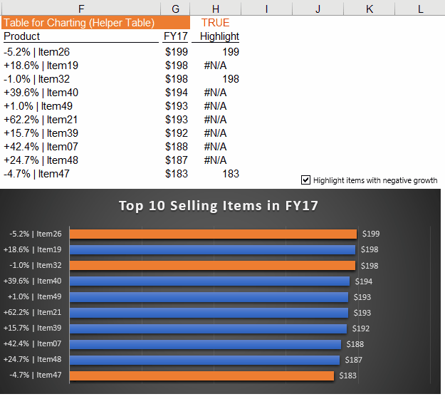
You boss loved it and asked… can you show also the 11th, or 12th…… even to the 50th items?

Yes, we have a total of 50 items in total in the data.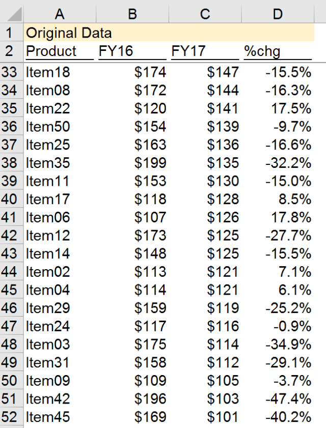

Let’s add a scroll bar to enhance this interactive chart so that user can scroll to see all the items if they want (but 10 items in a time).

In this post, I am going to show you how to insert a scroll bar and use the INDEX function to retrieve the data you need for the chart.

You may download a Sample File to follow through.

Setting up the (intermediate) helper table

Indeed, we will continue with the previous sample file, as we are building enhancement on top of it.  Make sense?

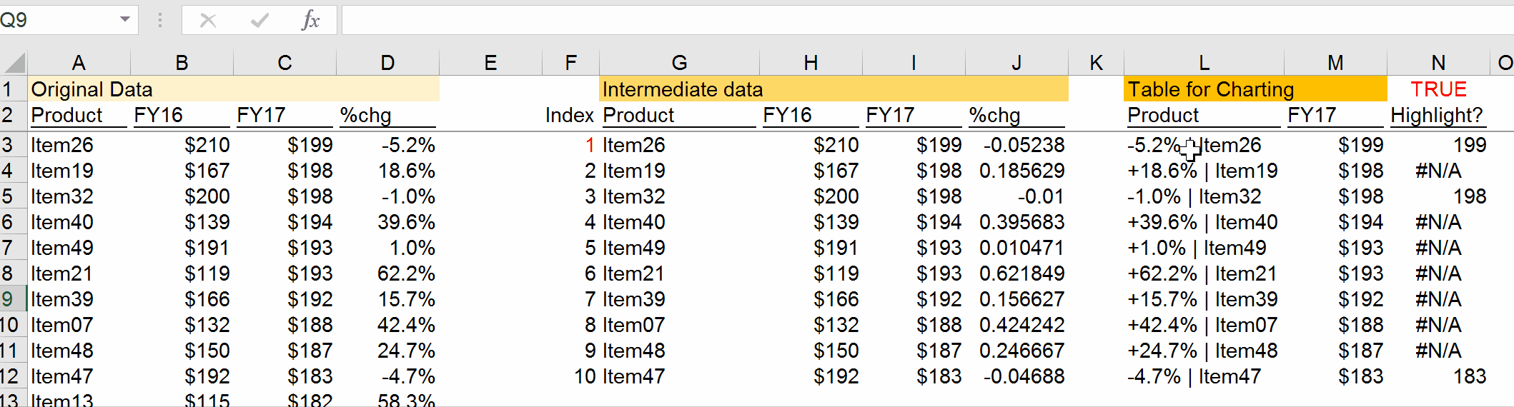
First, insert columns as shown below:

• Column F – index column for determining which rows of data to retrieve from
• Column G to I – getting the corresponding Product, FY16, FY17 data according to the index number
• Column J – a simple calculation of YoY % change.

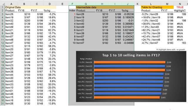
The following formulas are required:

In F3, input 1 (this will be the cell linked to scroll bar later)
In F4, =F3+1 'copy down to F12
In G3, =INDEX(A$3:A$52,$F3) 'copy down
In H3, =INDEX(B$3:B$52,$F3) 'copy down
In I3, =INDEX(C$3:C$52,$F3) 'copy down
In J3, =I3/H3-1 'copy down

Please pay attention to the mixed references; i.e. where the $ are.

Editing the formula in Table for Charting

The editing is easy.  Before, the formula were reference to the data source (Column A to D) directly.  Now we need the formula to reference to the (intermediate) helper table.

In L3, =TEXT(J3,"+0.0%;-0.0%") & " | " & G3 'Copy down
In M3, =I3 'Copy down
In N3, =IF($N$1,IF(J3<0,M3,NA()),NA()) 'Copy down

In case you do not want to rewrite the formula, you may do it with your mouse by drag and drop:

So far so good?

Inserting the Scroll Bar and adding control:

Now, we are ready to insert the scroll bar.

1. Go to Developer Tab –> Insert –> Scroll Bar (Form Controls)
2. Edit the Scroll Bar as shown below

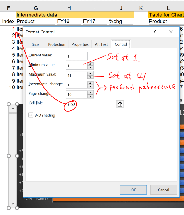You may refer to the basis of Form Controls for how to add a check box and assign linked cell.

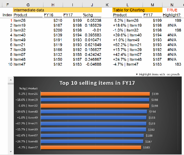
Here we go

Pls observe how the data (and chart) changes with the Form Controls.

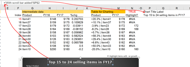
Are we all done?  Not yet.  Did you notice that the chart title is not making sense when we scroll down.  It is no longer Top 10…  The final step is to make the chart title interactive too.

Final touch up on chart title

In a blank cell, say P2, input the following formula to create an interactive chart title.

="Top " & $F$3 & " to " & $F$12 & " selling items in FY17"

The formula yields a result showing “Top X to Y selling items in F17” where X  (and hence Y) are determined by the scroll bar.

Then select the Chart Title, Click into the formula bar, Reference to P2

And we are done.  Happy weekend! 🙂

Final note: Using an intermediate helper table make the whole process much easier without complex formulation.