First of all, this blogpost is about Pie Chart, but not about how to make a Pie Chart.  Indeed, I am not going to show the steps of making Pie Chart here.   Also I am not intended to discuss whether Pie Chart is good or not to visualize data here. 🙂

One day my brother asked me how to show the data of “Jun” for the below Pie Chart: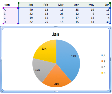

As you can see from the above screenshot, the data contains 6 series.  My question to him  was:  “How are you going to plot that into Pie Chart by using Paper and Pencil?”

A flash in my mind is something like this: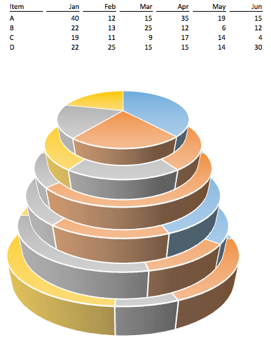

Seriously??? How are we supposed to visualize the data?

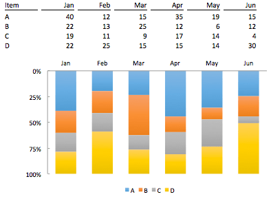
Joke aside, he just wanted something as simple as below:

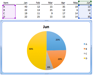
BUT with interactivity.

And you know what?  His chart was indeed a Pivot Chart.  I told him to use a slicer and simply select the month he needed.  Very simple.

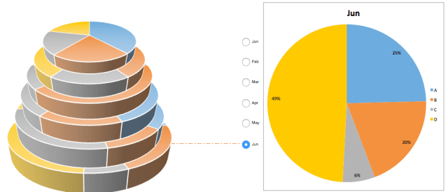
Nevertheless, that simple request inspired me to create a combination of Stacked (3D) Pies and 2D Pie to cater for his requirement.

So do you want some pies?

The Recipe:

• Ingredients: Pie Charts, Option button x 6, INDEX function, Icing sugar (Conditional Formatting), a little time and a little patience.
• Tools: Excel, what else?

The Making:

Stacked Pies

1. Start with the top-layer Pie: First to create a 3D Pie using Jan data
2. Trim all the ugly elements on your pie… e.g Title, legend, border, chart area and plot area (both set to no-fill)…
3. Duplicate the Pie using Feb data, make it a bit larger than the 1st Pie
4. Repeat above steps with Mar data, then Apr, May, Jun data one by one
5. Stack them with patience

Option Button x 6

• Go to Developer Tab –> Insert, Option Button.

Let’s try to make 2 buttons by following screenshots below to get a feel of it first.

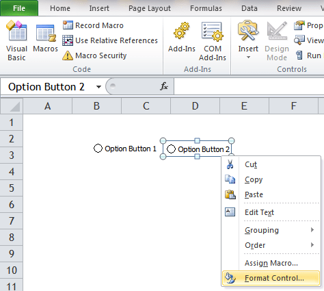(Right-click it)

 (Set Cell link to A1)

 (Try and observe)

• Got it?
• Repeat the steps to make 6 option buttons please.

After it is done, please set the cell link to $M$1, where underneath we are going to put the dynamic data to. (Tip: You may make one first, then set the cell link to $M$1, and then copy the Option button and paste 5 times)

The Dynamic data range

• In M2, input

=INDEX(C2:H2, $M$1) 'Copy down to M6

Now you should have your data set up as below: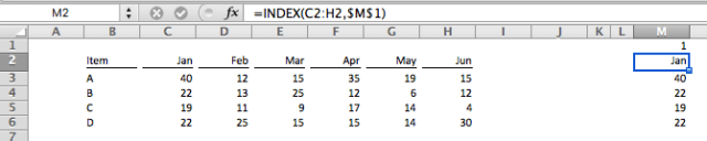

(Note: The value in M1 depends on which option button is selected… try it out)

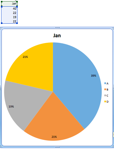
The Dynamic 2D Pie

• Simply create a 2D Pie using the data from M2:M6

Tidy up the dish

• Now we have all the key elements.  Just make them look pretty
• This should you how it looks like…

Final touch – Putting the icing sugar

• Select the cells in between the 3D pie and the option button
• Set Condition Format based on cell value in $M$1

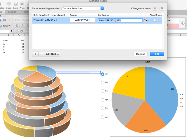
• Repeat for 2nd to 6th buttons. (Note: change the formula for conditional formatting accordingly).

The final product

Taste good!?  I hope you enjoy it.

You may download the sample file to follow through.

Guess if had done this for my brother finally?

No.  I didn’t.

Instead I propose the simple stacked column (shown below) to him and he seemed to be happy with that.