
We know that SUBTOTAL allows us to perform some basics functions like SUM, COUNT, AVERAGE, etc. that apply to visible rows only. However, there is no similar function for visible columns only.
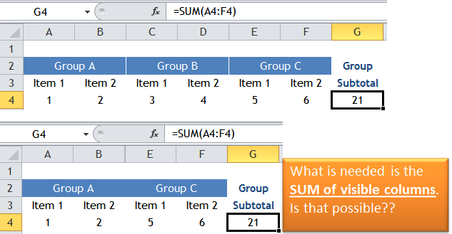 If we need to SUM visible columns only, we will need a twist.
The twist is not difficult at all. What we need is a helper row, say Row 1 in our example, and SUMIF function.
In A1, input the formula:
=CELL("width",A1) 'copy across to F1
As mentioned in previous post, the function CELL(“width”,A1) returns 0 (zero) when the column is hidden.
In G4, instead of a simple SUM, let’s do a SUMIF:
=SUMIF($A$1:$F$1,">0",$A4:$F4)
It simply instruct Excel to sum the range of A4:F4 where corresponding cells in A1:F1 is greater than zero (“>0”). Put it in other words, SUM visible columns only. YEAH!
Now we may hide column C:D to see the result…

Wait! It is still 21. Nothing change.
Unfortunately, this is the limitation. Although CELL is a volatile function (meaning it will get recalculated whenever there is a change in the worksheet), a simple HIDE/UNHIDE COLUMN action does not trigger recalculation. We need to give it a little push, say pressing F9, after hiding/unhiding columns.

(note: we may hide ROW 1 for better visual effect)
To further workaround it, we may GROUP columns and use the +/- button on the top to hide or unhide columns.
Please follow the steps below:
1) Insert 3 empty columns (C, F, I) (tips: set column width to 2 which is more or less the width of the +/- button displayed on top)
2) Select columns A:B

3) Data tab –> Outline Group –> Group (shortcut tip: Alt+Shift+Right arrow)

Now we should see the +/- button on top of column label
4) Repeat Grouping to columns D:E, and G:H (tips: Select the columns and then press F4, which is to repeat previous action)
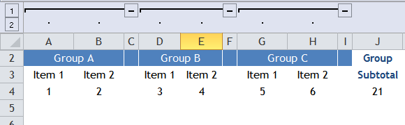
We should be able to get the above layout. Note: as we have inserted three columns, the formula in J4 (which was previously in G4) is now extended to cover column A:H.

Interestingly, hiding/unhiding columns by using the +/- button does trigger re-calculation.

With this workaround, we save the key stroke of F9 after hiding / unhiding.
Nevertheless, doing the GROUPing is kind of tedious. Moreover, it may not be easy to group columns with real life data in a seamless way without adding extra columns.
Therefore I would do this trick without GROUPing columns; but bear in mind of the F9 key. 🙂
Here is a Sample File for you to download.
What do you think about the trick? Please share with us by leaving comment.


Hi,
Neat trick!
However when I tried this in excel 365 it gave me a SPILL error
Is there any way out
As a corollary is there any other formula that will give a value only for visible rows like the CELL function so that we can use this method?
LikeLike
Hi Munshi, the SPILL error in Excel 365 means something is blocking the the way for the results to be spilt. Make sure you don’t have values on the right or underneath the active cells.
If you want the trick for visible rows, SUBTOTAL is a nice option. Pls refer to this post:
LikeLike
You can use sum function before the said formula.
=Sum(cell(“width”…
LikeLike
I used your formula but it returned incorrect results. It is difficult to explain what happened without sending an example spreadsheet, but essentially numbers from other cells which were not included in the specified range, were added to the sum. Note that this is nothing to do with hiding or unhiding columns.
I couldn’t pin down what was going on, though I did find a fix–which works—but I can’t explain why. The fix was to change =SUMIF($A$1:$S$1,”>0″,D3:R3) to =SUMIF($D$1:$S$1,”>0″,D3:R3). Only columns D-R contain numbers to be summed. However, changing to =SUMIF($B$1:$S$1,”>0″,D3:R3), or =SUMIF($C$1:$S$1,”>0″,D3:R3) in each case gave different but also erroneous results, which appear to include results from columns T,U and V in some combination, though they are not included in the range summed.
LikeLike
Hi Phil, the problem should be coming from the different range of columns you input int the first and final arguments. Why they start from different columns?
LikeLike
Pls also take a look at this post. It helps you better understand it. Hope this helps.
LikeLike
Thanks for that. I have not worked it through in detail with my example, but I am certain that is the explanation. A useful lesson…and thanks again 🙂
LikeLike
Thanks for this, which explains where I was going wrong. I did reply earlier to say thank you, but nothing seems to have been posted so I’m trying again1
LikeLike
You are welcome. Glad to hear that you find it helpful! 😉
LikeLike
Nice solution! I tried to google on Chinese and Japanese resources, but there is no Column’s solution (only subtotal 109 for ROWS). But once I tried to Google on English, I found your website 🙂 Thank you.
LikeLike
Thanks. Glad it helped! 😀
Btw i also have a YouTube channel where I have video in Cantonese…
check it out: https://www.youtube.com/playlist?list=PLnHdEIR8UL5OYDlQgnd30kBEV7Q30nx1X
😆
LikeLike
Nice trick!
Another twist to it is if you want to sum non-sequential visible columns only.
Instead of
=CELL(“width”,A1) in A1, you could put
=IF(CELL(“width”,A1)=0,0,1) which would put 0 in non-visible cells and 1 in visible ones.
You then need to sum like this:
=(A2A$1)+(C2C$1)+(E2*E$1)+…
And copy to all subsequent rows.
Voila!
LikeLike
Oupsss….I meant :
=(A2A$1)+(C2C$1)+(E2*E$1)+…
LikeLike
For some unknown reason, the star does not show in my reply in the first 2 brackets, so i will replace with x:
=(A2xA$1)+(C2xC$1)+(E2xE$2)+…
LikeLike
Hi Stephan,
Thanks for your comments and ideas… i guess the word editor of WordPress “eat” some special characters like ⭐️, smaller, larger… 🤔. Thank you for your patience to leave your messages. Appreciate it.
Btw, you may use SUMIF for an easier formula construction i think.
Cheers,
LikeLike