A simple but practical tip of using Advanced Filter

I came across a blogpost from Jon of Excel Campus (one of my favorite Excel sites) last week.  In his post, he showed how to filter for a list of items using a reverse partial match lookup.  Obviously, it is a formula approach.  From his post, you will see how Excel formula can save you from tedious works at workplace.

In this post, I am going to replicate Jon’s example and achieve similar results without a single formula.  Thanks to Advanced Filter!

Where is Advanced Filter?

Yes.  It’s right there – just next to the Filter that most people have used it.

But… I believe there is a high chance that you may have never used it before… 🙂  If that’s the case, please continue to read and you will find it super helpful.

Although with the term “Advanced”, Advanced Filter is indeed not difficult to use at all.

You may download a Sample File here to follow through.

Situation

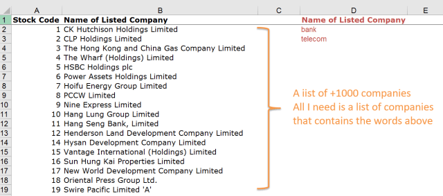
What we have is a list of 1000+ company names.  What we need is a list of companies that contains the word “bank” or “Telecom”.  You may wonder why we don’t just do it with normal Filter….

How to do it with a Filter?

1) The silly way

As I said, it is a tedious work.  Some people will browse the list from the filter and click the check box one by one, by eyeball.  Yes by eyeball.

Seriously?  No way… @_@

2) Using the Search box in Filter

Well, if you are an experienced user of Filter, you know that you may search for what you need by inputting the key words in the search box.  See below:

While you input “bank”, you will see immediately the filter is smart enough to show you only items that contain “bank”.  What’s is even better is you can ADD other search terms to your filter list – by checking the “Add current selection to filter“.

WOW, that’s good enough you may think.  Well… if we are dealing with only two items, yes it is.  Think about you need to deal with 10 items?  Then you need to repeat the steps 9 times.  That is tedious.  What’s worse?  The frustrating moment comes when you forget to check the “Add current selection to filter” on your final search term.  You know what I mean.

3) The proper way – Advanced Filter

Setting up

Before it works, we need to set a “Criteria Range” to tell Excel the list of names that we want.  Let’s set the Criteria using D1:D3

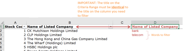
Note: The title of the Criteria Range, i.e. D1 in the above example, must be identical to the tile on the column we want to filter, i.e. B1 in the above example.

In action

Go to Data tab –> Sort & Filter –> Advanced

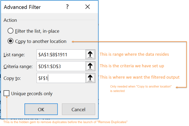
For demonstration purpose, I select “Copy to another location”.  You may, of course, “Filter the list, in place”, i.e in the original source location.

Here we go…

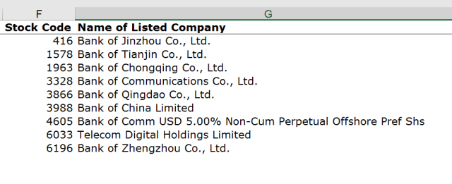
Wait… the matching list should be longer…

Apparently, the Advanced Filter only retreturnsmpany names that begin with “Bank” or “Telecom”…

A little twist – Using wildcard *

By wrapping the text string with asterisk (*), Excel now interprets the criteria as anything that contains “bank” or “telecom”.

Tip: * is the wildcard for any number of characters

Here we go…

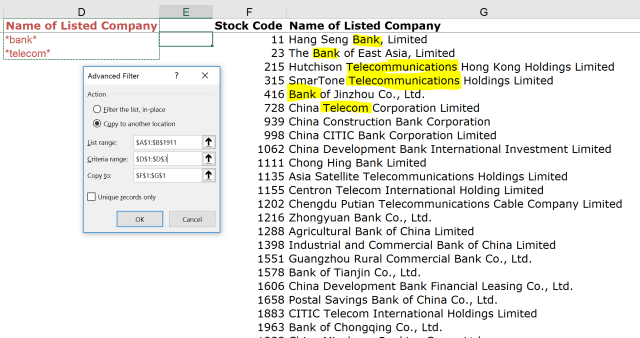
It is done and as simple as this…… if you need a partial match.  What if you want to differentiate Telecom from Telecommunications?

As you see from the above result, company names with “Telecom” and “Telecommunications” got filter altogether.  Indeed, that is what we instructed Excel to do… filter those contain the text string “telecom”.

To get the names with the word “Telecom” but not “Telecom*”, you will need an intermediate step.

Another twist – Adding space before & after the text string ” Telecom “

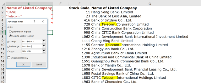
This simple twist instructs Excel to look for (space)telecom(space).  With this trick, the word “telecommunications” does not match the filter criteria.  Of course, this twist assumes each word be separated by space.

So are we done? Not yet… as the trick also excludes two possible scenarios:

1. Names start with “Telecom “
2. Names end with ” Telecom”

Here comes the Advanced part

To cater for the above scenarios, we need to add two more criteria into B4:B5.  That means we need to extend the Criteria range to D5.  See below:

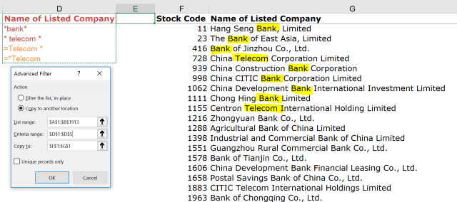
Note: In the sample file, you will see the filtered result at the end with two dummy names, one starts with Telcom; one ends with Telcom.

To be exact, the following are input as criteria:

B2 - *bank* 'Contains the string bank (any position)
B3 - * telecom * 'Contains the word telecom (in between only)
B4 - ="=Telecom *" 'Starts with the word Telecom
B5 - ="=*Telecom" 'Ends with the word Telecom

The input for B4 and B5 are not straightforward.  Nevertheless, once you learn the construction and do some practices, it will turn into another piece of cake… 🙂

To Recap

If you need to filter for a list of items (strings) regardless position in the source data, i.e. partial match, you may use Advanced Filter to do the job easily, as long as you remember to put * before the strings in your criteria range.  E.g.

*bank
*telecom
*technology
*holdings

However, if your requirement is a bit complicated, you may need to know the special construction for

="=ABC" 'Contains ABC only
="=ABC*" 'Starts with the string ABC
="=*ABC" 'Ends with the string ABC
="=ABC *" 'Starts with the word ABC; note the space
="=* ABC" 'Ends with the word ABC; note the space

Final note: Advanced Filter is case-insensitive

Please download the Sample File to practise.