
Did you know, you can plot a Waterfall chart in #Excel in less than a minute…Provided that you are using Excel 2016 or later! 🙂
No Kidding! You may download a Sample File to follow along.
A) Data layout

Note: The ending value should be computed with a simple SUM function.
B) Plot the chart
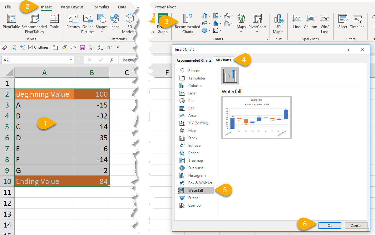
- Select the range of data
- Go to Insert tab
- Click Recommended Charts
- Go to the All Charts tab
- Select Waterfall
- OK
You should get the following waterfall chart.
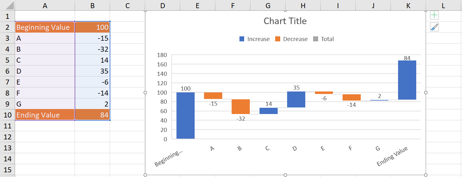
Yes. You are right, the ending column should not be like that…
No worries. All you need is just a few more clicks.
C) Setting the total column
Again, a picture tells a thousand words…
Note: The first click on the column will select all columns. You have to click again to select a single column, followed by right-click on it to open the menu.
D) Optional, let’s do some makeup (formatting)
Here you go!
Bonus – How about when I have subtotal?
You won’t believe how easy it is. Watch this:
As simple as this. 😀
You may watch it in action in my YouTube channel too:


Hey, I found your article interesting and insightful. I was just wondering if you can give your thoughts and your 2 cents on how to improve this article?
https://www.efinancialmodels.com/knowledge-base/excel-google-sheets-co/excel/how-to-create-a-waterfall-chart-for-excel-financial-models/
Thank you so much!
LikeLike