Don’t be shy!  Let silly things continue!  Let’s Hide and Seek with #Excel again! 🙂

Case 1

Case 2

Case 3

You may download a Sample File – Hide and Seek Cell Content for the above cases.

If you know the answers to all the three cases above, I believe you are good at using Excel.  If you don’t know all of the above, you may want to continue.

Case 1 – The most common scenario

The text is always there… just that the font are formatted in the same color as cell fill color. Well, it’s true that a normal person does not see white on white.  Excel Humor #9 – You do not see me

Tip: The “disappeared” middle gridlines from D3 to I3 is a good indicator for this scenario.

Solution

To make the cell contents visible to normal person, simply change the font color:

Case 2 – A very special custom format to hide cell content

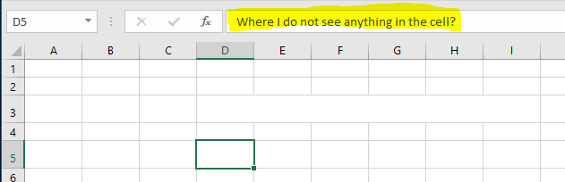
Similar to the “hidden” content in D3, but in this case the font color is Black.  Also, the middle gridlines from D5 to I5 are there.  Does it mean that cell D5 is really empty? Should not be… as we can see the content in the formula bar.

Strange enough?  It is due to Custom Format.

Solution

Simply change the cell format to “General”

Curious about the Custom Format that hides cell content?

Here you go:

Format Cells –> Number Tab –> Custom (under Category:) –> Type: Three semi colons as followed:

;;;

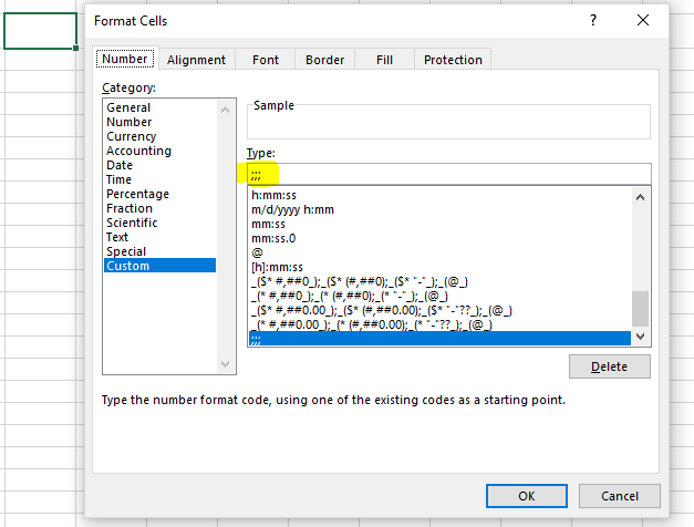
Note: This custom format does not hide #ERROR!.

p.s. I love this trick! 🙂

Case 3 – A reversed case

In this case, we see the content in a cell but not in the formula bar… how come?

Try to click into the formula bar, and you will see the following error message:

The cell or chart you’re trying to change is on a protected sheet.  To make a change, unprotect the sheet.  You might be requested to enter a password.

It is absolutely normal if you do not know you could protect a formula (or cell content) from displaying in formula bar.  To do so, we simply need to

Format Cells –> Protection tab –> Check the “Hidden” box

Note: It takes no effect until you protect the worksheet.

Solution

Obviously, the solution is simple: Reverse the above steps by unprotecting the worksheet (provided that you know the password, or there was no password set.)

What if…… we do not know the password?

Easy… Add a new worksheet, or go to a worksheet that is not protected, input the following formula in an empty cell.

=FORMULATEXT(SheetName!D3)
where D3 resides the formula you want to look into.

If #N/A is returned, it means the origin content in the cell is a text string or number as you see it.  It is not a result from formula.

Note: FORMULATEXT function is available in Excel 2013 or later versions.

What?  Still using Excel 2003??????

Why not copying D3 and paste on an unprotected sheet?  Isn’t it the simplest way? 🙂

What? You cannot copy D3 as the worksheet is strictly protected in a way that you cannot even select D3????

No worry.  Check this out: Copy data from strictly-protected sheet