I seldom use the HYPERLINK function in #Excel. Normally I insert hyperlink by CTRL+K, then setting the reference I want the link to go to. That is super easy (or quick and dirty)!

Note: You may go to Insert tab on ribbon –> Link
However, laziness comes with a price, i.e. limitation ==> Static link. We cannot insert different hyperlinks based on the contents in a range of cell. And that’s the reason I need the HYPERLINK function. Here’s my story:
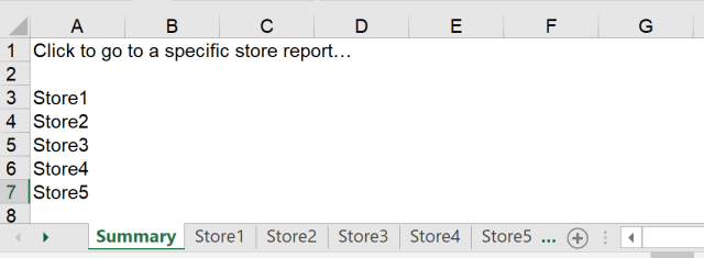
Recently, I created a workbook with more than 50 sheets. For easy navigation for users, I created a summary page, with a table of content. Well, 50 sheets! And I am not going to insert 50 different links by doing the CTRL+K 50 times. NO WAY.
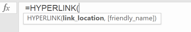
As I said, I seldom use HYPERLINK function and I did not remember the arguments for this function. I paid close attention to the hint while I typed =HYPERLINK in the formula bar…
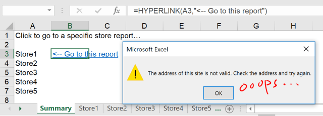
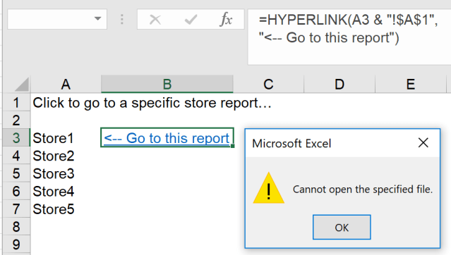
And this is my first attempt, a fail attempt…
I clicked the “fx” icon on formula for more details…
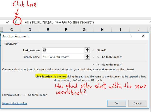
Although I realized that I need to input a text string for the “Link_location”, I was not sure how to do that for a location within the same workbook. Then I clicked “Help on this function” in order to find the correct way to construct what I need.
This is what I do for many functions… who knows all 400+ functions in Excel? Maybe there are someone but not me. 😛
Here’s what I get from Excel Help:
The Syntax:
- Link_location Required. The path and file name to the document to be opened. Link_location can refer to a place in a document — such as a specific cell or named range in an Excel worksheet or workbook, or to a bookmark in a Microsoft Word document. The path can be to a file that is stored on a hard disk drive. The path can also be a universal naming convention (UNC) path on a server (in Microsoft Excel for Windows) or a Uniform Resource Locator (URL) path on the Internet or an intranet.Note Excel Online the HYPERLINK function is valid for web addresses (URLs) only. Link_location can be a text string enclosed in quotation marks or a reference to a cell that contains the link as a text string.If the jump specified in link_location does not exist or cannot be navigated, an error appears when you click the cell.
- Friendly_name Optional. The jump text or numeric value that is displayed in the cell. Friendly_name is displayed in blue and is underlined. If friendly_name is omitted, the cell displays the link_location as the jump text.Friendly_name can be a value, a text string, a name, or a cell that contains the jump text or value.If friendly_name returns an error value (for example, #VALUE!), the cell displays the error instead of the jump text.
Good news is what I highlighted in red. The function works for jumping to a specific location in an Excel worksheet or workbook. Not too good news is it did not specify how…
So it’s better to look at examples… Because my objective was to create links within current workbook, I focused on examples demonstrating it…
| Example | Result |
| =HYPERLINK(“[Book1.xlsx]January!A10″,”Go to January > A10”) | To jump to a different location in the current worksheet, include both the workbook name, and worksheet name like this, where January is another worksheet in the workbook. |
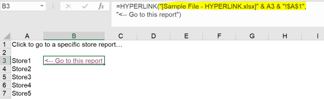
=HYPERLINK("[Sample File - HYPERLINK.xlsx]" & A3 & "!$A$1",
"<-- Go to this report")
'where A3 resides the sheet name;
Note: The ! after sheet name before cell reference is necessary
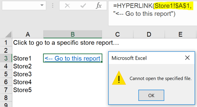
Exciting moment… Did it work?
| =HYPERLINK(CELL(“address”,January!A1),”Go to January > A1″) | To jump to a different location in the current worksheet without using the fully qualified worksheet reference ([Book1.xlsx]), you can use this, where CELL(“address”) returns the current workbook name |
Indeed, it was not about jumping to a different worksheet in the current workbook. Nevertheless it reminded me of the function CELL. After many semi-successful and fail attempts, I guessed I understood how HYPERLINK function works: I needed to feed a text string of file name + sheet name + reference into the first argument (i.e. Link_location). The challenge up to this point was to get the file name. There are many ways to do so. And I used the following formula:
=LEFT(MID(CELL("filename"),FIND("[",CELL("filename")),99),
FIND("]",MID(CELL("filename"),FIND("[",CELL("filename")),99)))
Then I put this into the first argument of HYPERLINK:
=HYPERLINK(LEFT(MID(CELL("filename"),FIND("[",CELL("filename")),99),
FIND("]",MID(CELL("filename"),FIND("[",CELL("filename")),99)))
& A3 & "!$A$1",
"<-- Go to this report")
where A3 and "!$A$1" are the sheet name and cell reference respectively
Guess what? It worked, finally!
As I did not hard-code the file name into the formula, I could save the file as new file name without worrying the links go wrong. 🙂
The story has not yet finished…
Although I had fixed my problem, I didn’t think that’s the right way as it was so stupid. I couldn’t believe there is no simpler way to achieve the same thing. So what did I do? GOOGLE! What else?!
The top search result was an article by Debra Dalgleish of Contextures , one of my favorite Excel resources site. I was very confident that I could find the answer I was looking for.
Here’s the missing link
With no doubt, I got what I needed from the article of Contextures. What I needed to do was to replace the long formula for getting the file name with #.
Before, my formula was:
=HYPERLINK(LEFT(MID(CELL("filename"),FIND("[",CELL("filename")),99),
FIND("]",MID(CELL("filename"),FIND("[",CELL("filename")),99)))
& A3 & "!$A$1",
"<-- Go to this report")
where A3 and "!$A$1" are the sheet name and cell reference respectively
After, my formula is:
=HYPERLINK("#" & A3 & "!$A$1",
"<-- Go to this report")
# is the trick. It means current workbook here.
Moral of the story:
- Google maybe more helpful than Microsoft in finding a solution of an Excel problem. 🙂
You may download a Sample File – HYPERLINK to experiment.


Thanks for the article, it was super helpful and informative!!!
LikeLike
You are welcome! Glad it helped! 😃
LikeLike
Thanks, very helpful. This is exactly what I was looking for as I wanted to create an electronic table of contents. I had to add one thing as some of my worksheets had spaces in their names. If you were to refer to that sheet in a formula it would be =’Sheet Name’!A1 so the formula needed to be changed to =HYPERLINK(“#”&”‘”&A3&”‘”&”!$a$1″,”<— Go to this worksheet”) when A3 contains that name of the worksheet you want to go to.
LikeLike
Glad it helps. And thanks for your input concerning space in worksheet names. 🙌
LikeLike
There is a link under (almost) every article on office.com/microsoft.com: “Was this information helpful?”
Click on “No” and explain yourself.
Click on “Send”.
Maybe it will help. 🙂
LikeLike
I did. And indeed that is the button I clicked many times. 😅
LikeLike