Got this question from my brother. He is tracking scores for game he plays with friends. The game can be played with up to four players. He wants a formula to calculate the last 10 scores of a player. He showed me the above layout and asked for the formula to SUM and AVERAGE the last 10 records of each player…… As he called me Excel guru, there is no reason I do not help him. 😁

For demonstration purpose, I change the last 10 records to 5. Indeed, I have assigned a variable (from 3-10) for user’s selection. The expected result is to obtain the SUM and AVERAGE of the highlighted cells, shown below:

And new records will come from time to time. That means the table will expand. The best way to deal with it is of course (not whole-column-referencing but) turning the data range into Excel Table.

You may download a sample file to following along.

Turn the range into Excel Table

Select the range of data, then go to Insert tab –> Table

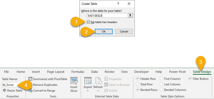
1. Confirm the data range and check “My table has headers“
2. Click OK
3. When the Table is created, go to “Table Design” tab
4. Give it a meaningful name. I’ve assigned the name “tb_Score“.

As simple as that.

Solving the problem

The problem seems complicating… indeed it is not, especially when there is a date column in ascending order AND nothing will be input if a player skips a game.

Tips: There are many different ways in solving a problem in Excel. Whenever we can, exam the contexts and understand the requirements before constructing the solution. It may help simplified the solution. 😉

Since there is a date column, we are going to use it to identify the starting point for each player. Once the starting point is identified, we can use SUMIFS (or SUMIF for Excel 2003 or before) to sum all the vales that is equal or larger than the starting point. Make sense?

To identify the starting point

This will be the major challenge of the problem. When it is solved, the rest should not be a huge problem.

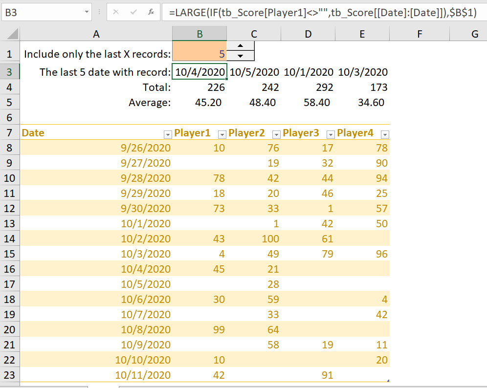
In B3, input the following formula:

=LARGE(IF(tb_Score[Player1]<>"",tb_Score[[Date]:[Date]]),$B$1)

Let’s examine the inner part of the formula:

IF(tb_Score[Player1]<>"",tb_Score[[Date]:[Date]])

Note: [[Date]:[Date]] lock the [Date] column in the table so that
it won't move to the right when the formula is copied to the right
This is the absolute form in structural referencing formula.

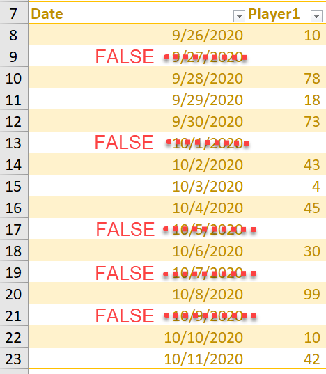
The above formula examines the date when the score is not blank. It instructs Excel to return a list of date when there is a score associated to it; “FALSE” when the corresponding score is empty.

When the inner portion of the formula got evaluated, Excel returns the following result:

=LARGE({44100;FALSE;44102;44103;44104;FALSE;44106;44107;44108;FALSE;44110;FALSE;44112;FALSE;44114;44115},$B$1)

Note: The number 44100, 44102, 44013, etc. are the numeric value for the date “9/26/2020”, “9/28/2020”, “9/29/2020”, etc. respectively.

Visually in a grid, it looks something like this:

The LARGE portion is easy, it takes two arguments:

LARGE(array, k)

Array    Required. The array or range of data for which you want to determine the k-th largest value.
K    Required. The position (from the largest) in the array or cell range of data to return.

=LARGE({44100;FALSE;44102;44103;44104;FALSE;44106;44107;44108;FALSE;44110;FALSE;44112;FALSE;44114;44115},$B$1)

Now it’s obvious that the above formula will give us the date where we have the last 5th score (the 5th Large number). The following screenshot gives a better illustration:

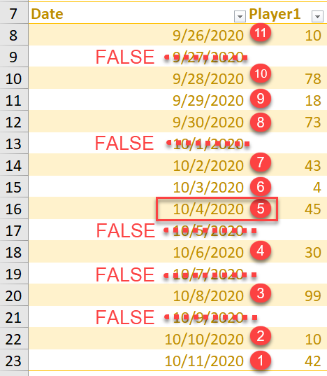
As a result, we have identified “10/4/2020” as the starting point to SUM all the scores afterward for Player 1.

SUM the rest using SUMIFS

In B4, input the following formula:

=SUMIFS(tb_Score[Player1],tb_Score[[Date]:[Date]],">="&B3)

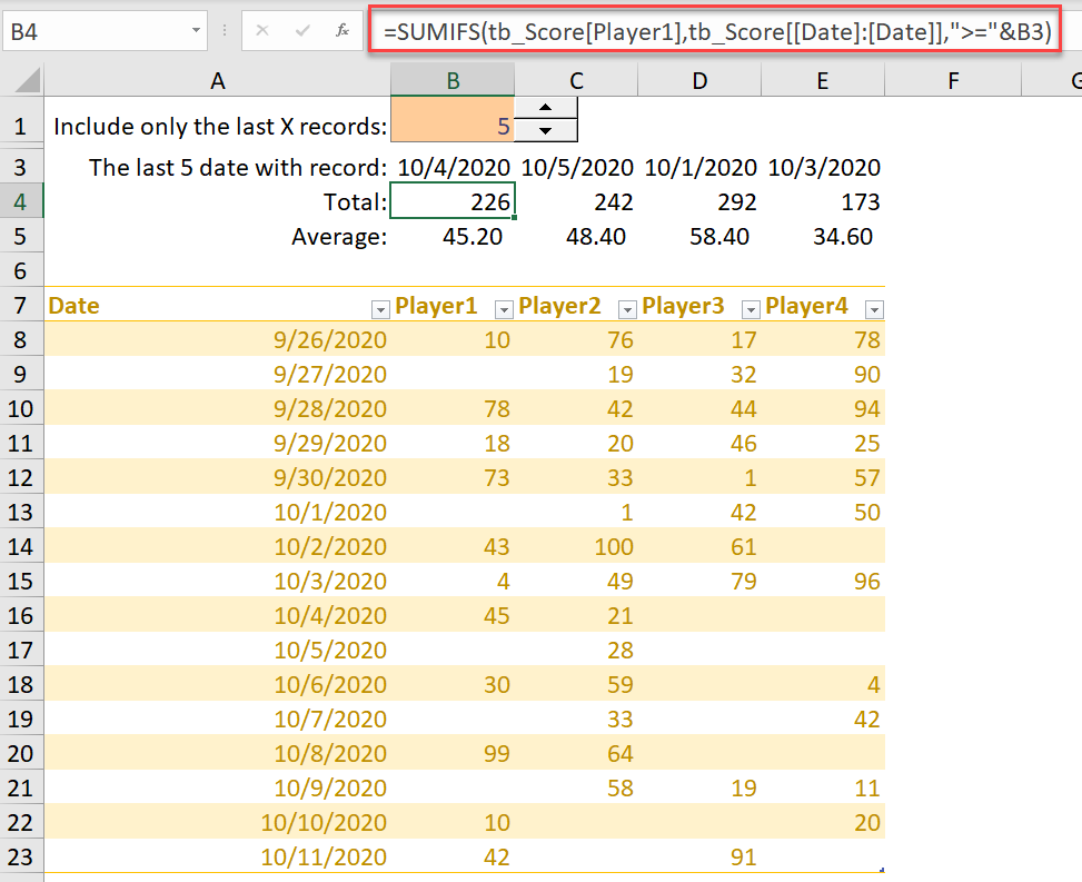
As Excel treats blank cells as zero, we don’t have to worry about all the blank cells in between. SUMIFS does the job to add the last 5 values correctly. 🙌

Getting the average

This should be the easiest part of the problem. We have the SUM, we have the number of incidents… To get the average, a simple formula would do. In B5, input:

=B4/$B$1

Final step – copy the formula to the right

If you want, you can combine the formula used in B3 into B4 and then get rid of row 3. However, I would simply hide row 3.

Don’t forget to download the sample file to try it. Do add some new records to the end of the Table and observe.

I hope you like it. 😉