Find and Replace is a very handy tool in Excel. It helps you to find a value quickly. You may then replace the value found with another value, either one by one or replace all at one batch.

To use the basic of Find and Replace, it requires no special reading as it is quite straight-forward. Perhaps the most practical tip to regular user is the shortcut keys:

• Ctrl+F ==> Find
• Ctrl+H==> Find and Replace

However, did you know… you can also

1. specify the search condition to look for “partial” or “exact” match?
2. ask for “case sensitive” search?
3. look into values only (not formula)?
4. even search for a format?

If you are eager to learn more about Find and Replace, and hence boost your productivity with Excel, please continue to read this article. 😉

You may download a simple file to follow along.

FIND (Shortcut: Ctrl+F)

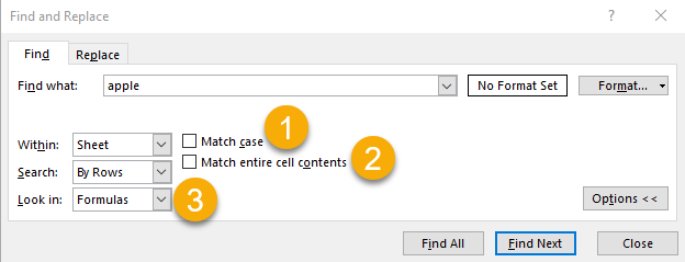
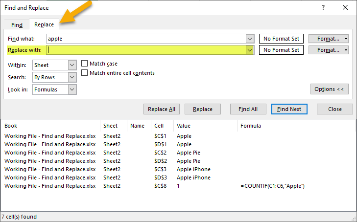
To start with, let’s understand the default setting of Find by using a simple example. Let’s open the Find dialog box by pressing Ctrl+F, followed by input “apple”, as shown below.

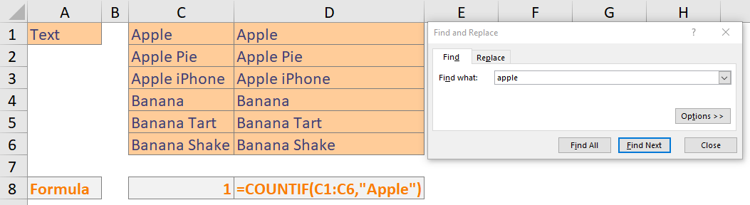
Clicking the “Find Next”, Excel takes you to the cells that contains the text string “apple” one by one, by row.

You may have already noticed that the search mode is by default:

1. partial match (searching cells that contain the text string)
2. case in-sensitive (searching “apple” would give you “Apple” too)
3. kind of strange… why C8 qualified the search?

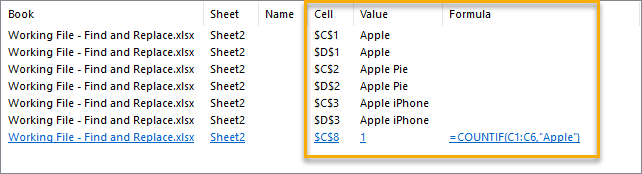
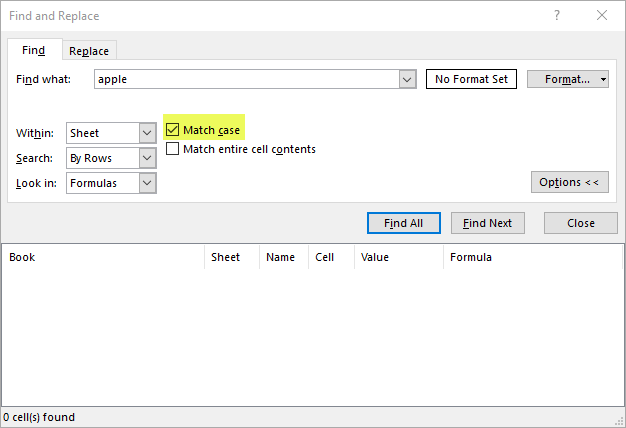
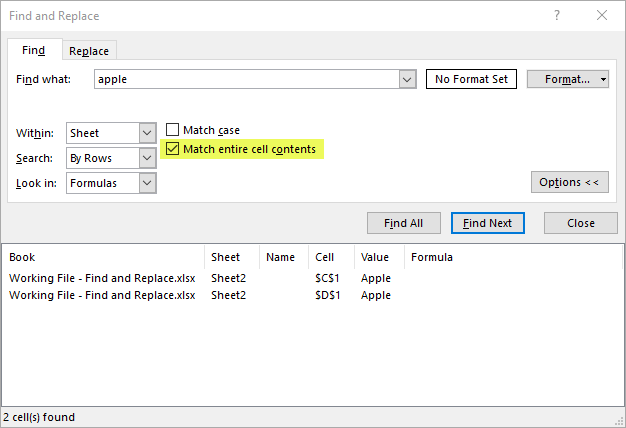
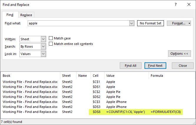
Now let’s see all the matched results by clicking “Find All“:

The cell C8 contains a formula

=COUNTIF(C1:C6, "Apple")

That’s why it fits the search criteria too and C8 is returned as one of the results. Pay attention to the results in the “Find” dialog box. C8 has a value of “1”, which is the result from the formula that contains the text string “apple”.

The behavior is resulted from another default setting of “Look into formulas”.

So far, I’ve talked about three different settings:

1. Partial match or exact match
2. case sensitive or case in-sensitive
3. look into formulas

So, where can we see these setting? 🤔

It’s time to click the “Options>>” – a button that appears in different occasions but got ignored most of the time… 😔

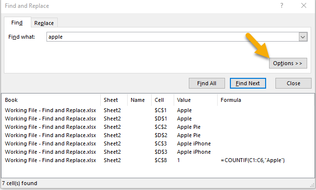
When we opened the Options, we will see the settings we just mentioned:

When “Match case” is checked, no cell is found with “apple” because we instructed Excel to do a case-sensitive search.

When “Match entire cell contents” is checked, only two cells (C1 and D1) are found as they fulfill the condition of “exact” match (regardless of case when the “Match case” is unchecked).

When we changed the Look in from “Formulas” to “Values“, C8 is no longer a match but D8 is. Why? Because the value of C8 is 1 that does not contain the text string “apple”. On the other hand, the value of D8 (resulted from a formula) contains the text string “apple”.

There are indeed more options we can select from:

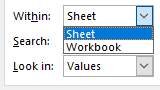
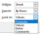
These options are intuitive.

1. We can limit the search to the current worksheet, or extend it to the entire workbook.
2. Search either by rows or by columns. It has impact on the display order in the “Find All” results; or on the sequence of “Find Next”.
3. We can look into formulas, values (the subtle difference was described above), Notes (formerly known as comment in older versions of Excel) or Comments.

Didn’t know there are so many options for FIND? You are absolutely normal, from my point of view. Last but not least, I would like to draw your attention to the last option available… probably the least noticed option: Format…

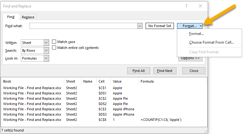
When we click the “Format…“, here we go:

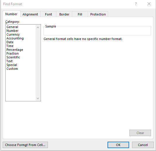
Does it look familiar?

Yes!!! Of course, that’s the Cell Format dialog box. But here, we specify a format to look for. It could be easy to select a yellow filled format. However it is not at all easy to select a format we see on a worksheet. Here comes the “Choose Format From Cell…” to rescue.

In the above screen cast, you see how we we find cells with a specific format using “Choose Format From Cells…“.

Note: I have cleared the content in the “Find what:” box (nothing there). If you have input “apple”, you are then searching cells that contains “apple” with the specific format (note: this is in effect an AND condition)

REPLACE what have been found

When we know how to find what we want precisely, it’s piece of cake to replace what have found with a specific value, with or without a specific format.

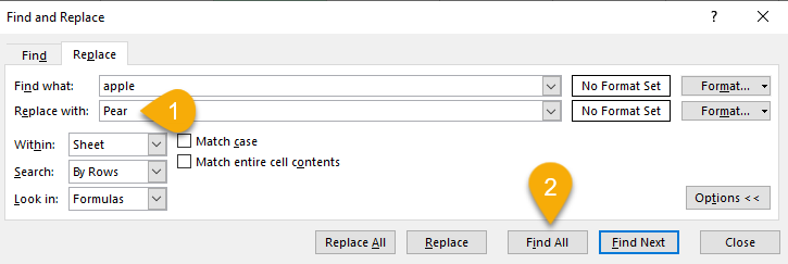
Let’s try to replace “apple” with “Pear”

1. Input “apple” and “Pear” into “Find what:” and “Replace with:” respectively
2. Click “Find All”

Note: You can click “Replace All” directly, if this is what you want to achieve

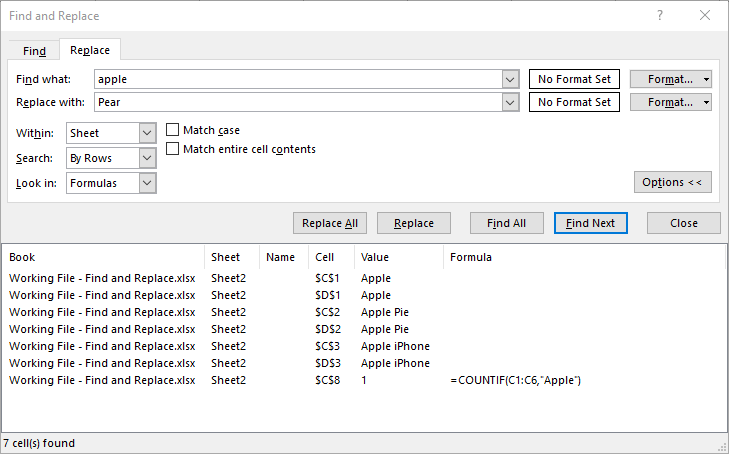
We can see the results in the lower part of the “Find and Replace” dialog box. Indeed we may navigate to a “found” result by clicking on it.

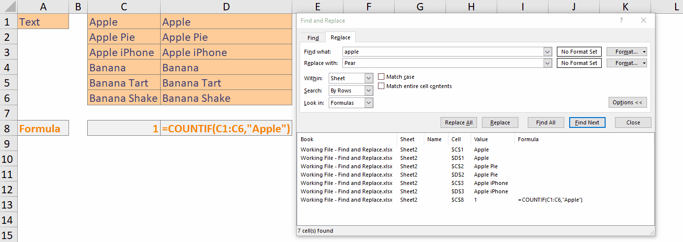
By doing so, we can replace the value in selected cell(s) only. For example, replacing “apple” with “Pear” found in formulas only:

Isn’t it nice? 😻

If we want to replace all the “apple” found, simply click “Replace All“.

Tip: You may specify a range to perform the Find and Replace action. Select the range on the worksheet before staring the Find and Replace. It may be helpful if you are working with a huge workbook but only focusing on a relatively small range of data.

Here’s a short video to show you how to Find and Replace a format:

I hope you like it.

How do you using “Find and Replace”? Please share with us by leaving comments below.