Interesting application of Power Query for real life problem – See how to transform table into different layout using Power Query

I came across this Power Query Challenge from Computergaga and I found it really interesting as it seems that it happened to some of my ex-colleagues for event planning before.

I took the challenge.  In this post, I will give a possible way of solving it with Power Query.  Yes only one of the possible ways.

The Challenge

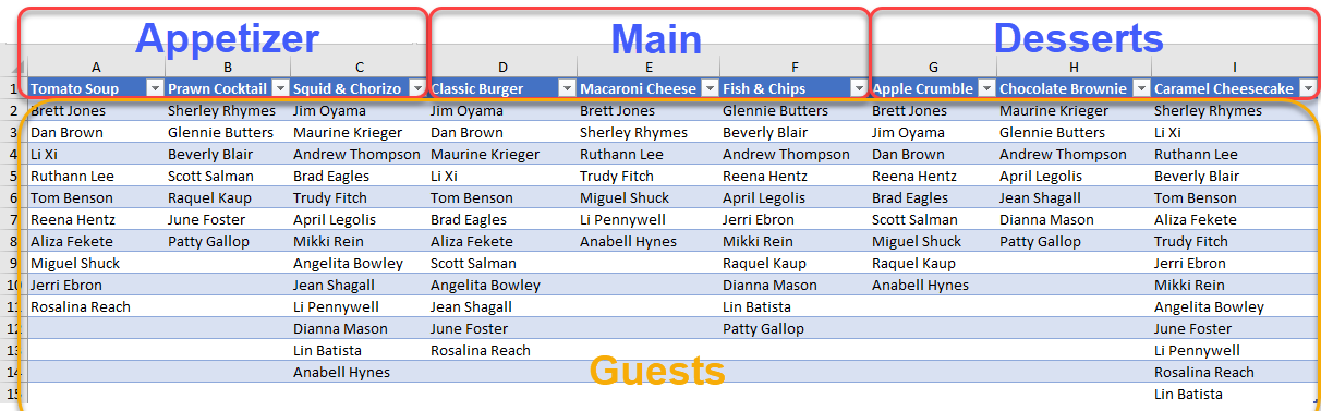
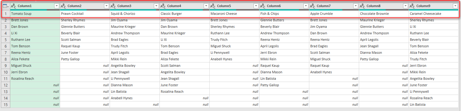
You’ve got the following table. The headers of columns are different types of dishes that your guests can select from.  What underneaths are the guests who pick it.  The first there columns are Appetizers, while the middle three and the last three columns are for Main course, and Desserts respectively.

Is the above a bad layout?  Well it depends.

If you serve the dinner, it works fine as you know exactly which dish goes to which guest.

However, if you are the event planner and you want to confirm the dishes selected by your guests, this above table is a nightmare to you.   Isn’t it? 😂

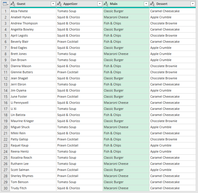
What you would like to see should be a table like this:

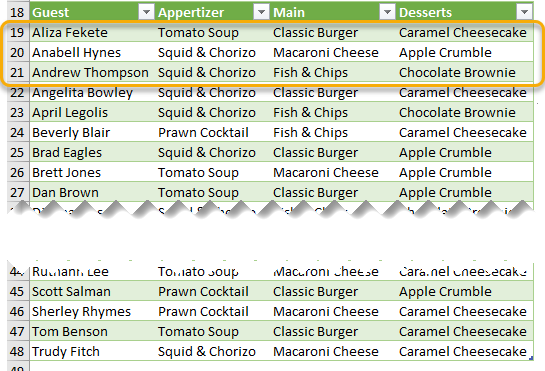
It clearly states who eat what (as appetizer, as main and as dessert).  It will certainly save your day! 🙂

And this is exactly the expected result #1 of the challenge.

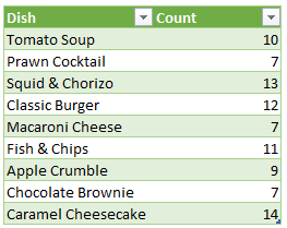
Expected result #2 is more for the kitchen member, I guess.

They are more concern on the quantity of each dish.  They don’t (usually) care who eats what?  They just want to know the quantity required.  The following summary table will do.

If you want to watch the original video for the challenge and the solution from Computergaga YouTube channel, please click HERE. You can get the sample file to follow along from there too.

My solution

Here’s my approach to solve the problem

1. Generate a unique list of dish and identify if it is a appetizer, main or dessert.  Luckily the data is not too bad; they are all grouped together with a constant number. (otherwise, we may need a helper table to do so)
2. Transform the source table with transpose and un-pivot
3. Merge the result table with Query 1 to identify the type of dish
4. Pivot it to get the final table… desserts time. 🙂

You may download a sample file with the queries at the end of the post.

Note: All screenshots used in this post are captured using Excel for Office 365.  If you are using other versions of Excel, you may find the locations and look&feel of buttons a bit different. The concept is the same though.

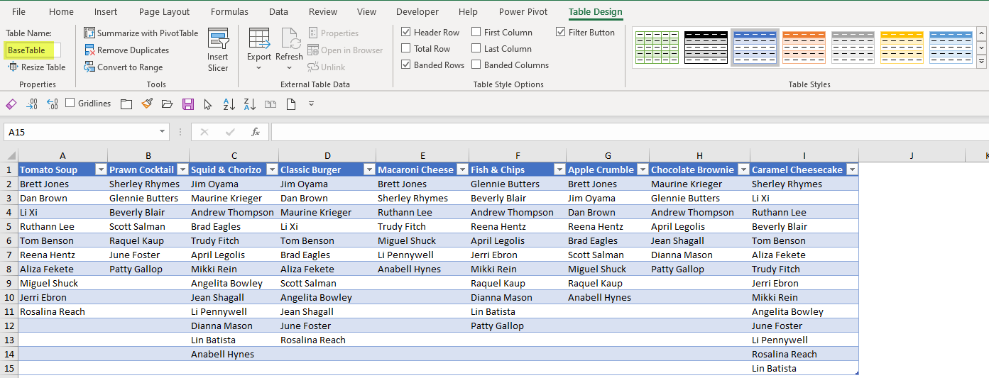
First thing first, Convert the data range into an Excel Table

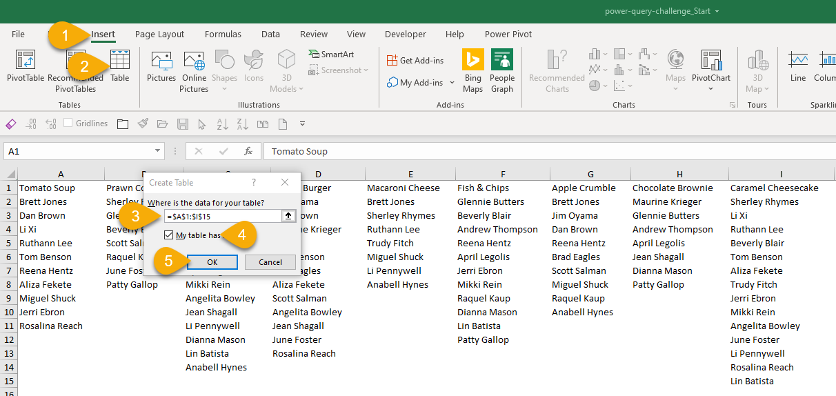
I named the Table as “BaseTable” which is our starting point.

A. Load “BaseTable” to Power query

• Select any cell of the BaseTable

1. Go to Data tab
2. Select From Table/Range

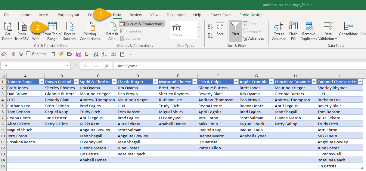
The following Power Query Editor opened.

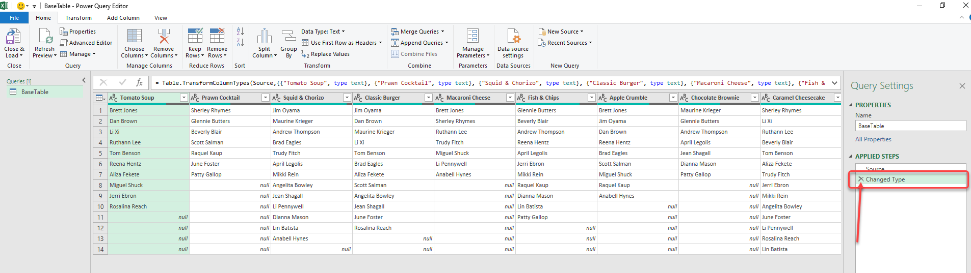
Note: the Query Name is the same as the Table Name.  You may revise it if you need.

The Query Settings pane on the right shows all steps we applied to the query.  Now, let’s remove the step “Change Type” by clicking the X next to it.

Now, we demote the header to get the list of dishes.

1. Go to Home tab
2. Click the dropdown menu of “Use First Row as Headers“
3. “Use Headers as First Row“

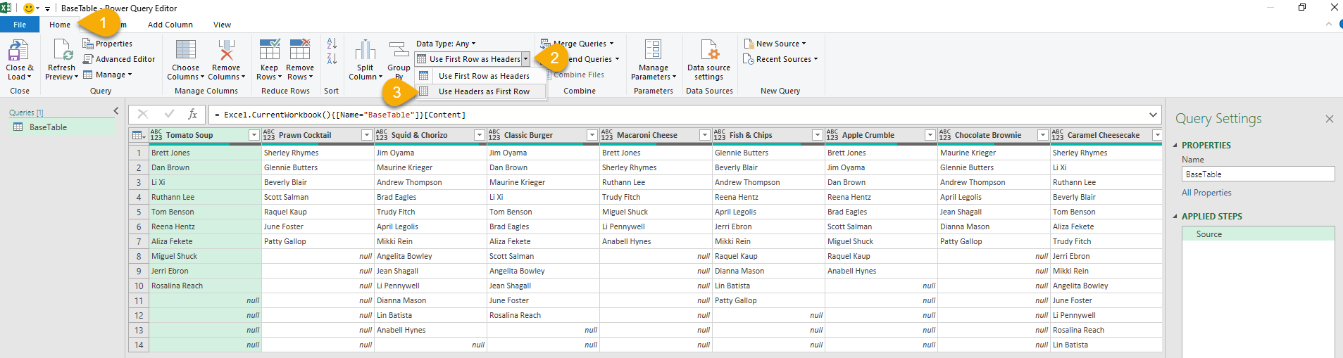
Now we have all the dishes on first row:

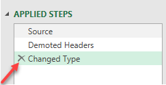
Let’s take a look at the Applied steps on the Query Settings Pane.  The last step “Changed Type” was generated automatically.  We don’t what this step, so let’s remove “Change Type”

Well, we have set the BaseTable, we can continue to build our query based on it.

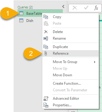
B. Create a new Query by referencing the BaseTable, and to prepare a list of dish identifying appetizer, main, dessert

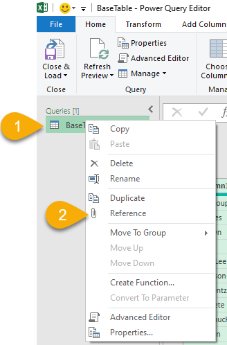
Open the Queries pane on the left,

1. Right-click “BaseTable”
2. Select Reference

Now, we should see the following, which is exactly the result of the last step of “BaseTable“.

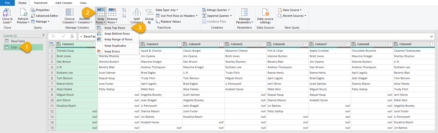
1. Let’s rename it to “Dish” (by right-click on “BaseTable(2) and then rename)
2. On the Home tab, select “Keep Rows“
3. Keep Top Rows

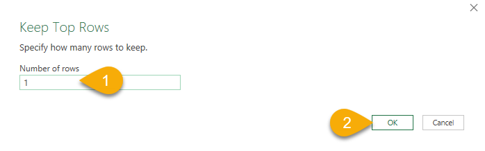
In the dialog box,

1. Input 1 in the “Number of rows”
2. OK

By now, we should be seeing on the top row that lists all the dishes.  Let’s transpose it to a column:

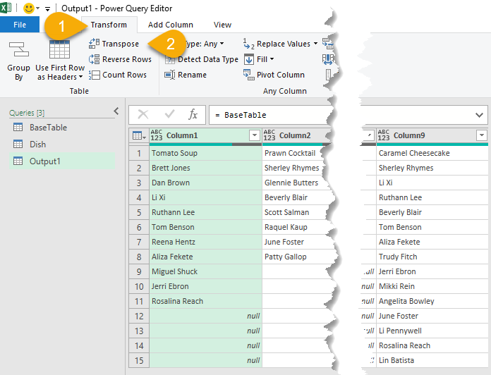
1. Go to “Transform” tab
2. Transpose

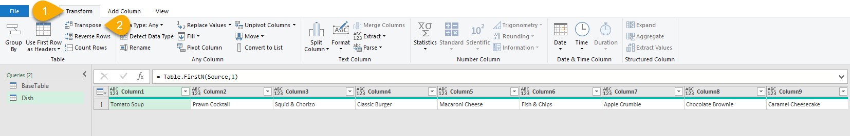
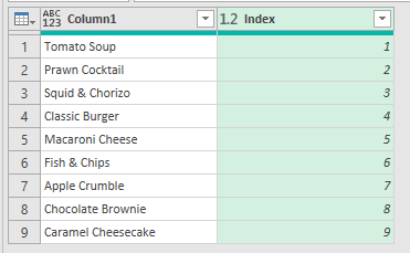
Here we go:

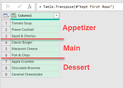
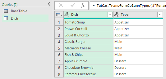
We have nine different dishes in total.  The first three are Appetizers, the middle three are Mains, and the final three are Desserts.  Cool.

Let’s Add an Index Column:

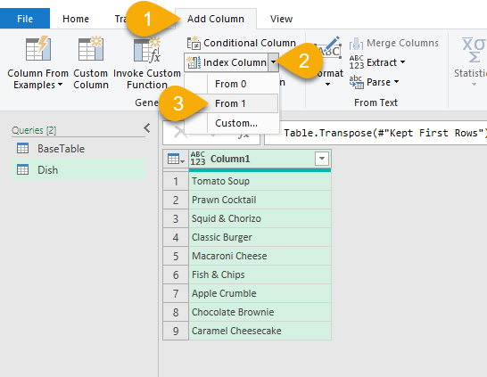
Here we go:

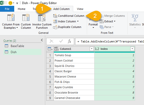
Indeed, I want to label the first three rows as Appetizer, the middle three as Main and the final three as Dessert.  To achieve that, adding a Conditional Column is a simple way (given we don’t have many items).

1. Go to Add Column tab
2. Conditional Column

Input the following from the “Add Conditional Column” dialog box:

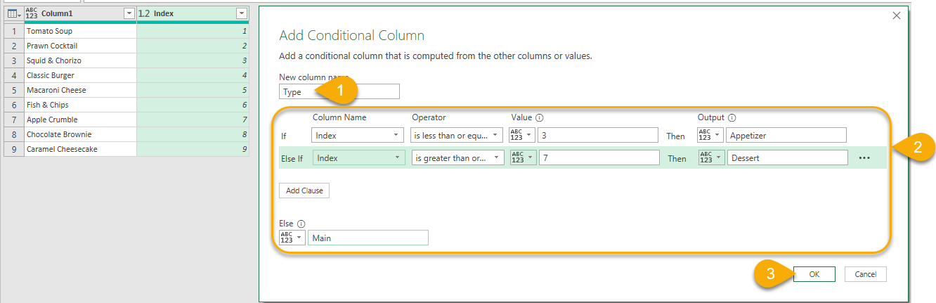
1. The name of the new column, where I input “Type“
2. Conditions – where Index is less than or equal to 3, they are “Appetizer“; where Index is greater than or equal to 7, they are “Dessert“; everything else is “Main“.  Make sense?
3. OK

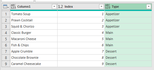
Here we go!

Let’s do some tidy up to conclude this query:

Tip: To select multiple columns and apply data type together, hold Ctrl key

This is the result of the query “Dish“.  We will use it later.

C. Create the Output1 query where magical transformation happens

1. Right-click the “BaseTable” query
2. Select Reference

Rename the BaseTable(2) to Output1

Now, we are ready to Transpose the Table

1. Go to Transform tab
2. Transpose

When the Table is transposed, we see that all “Dish” are now under Column 1, where all guests are in the subsequent columns.

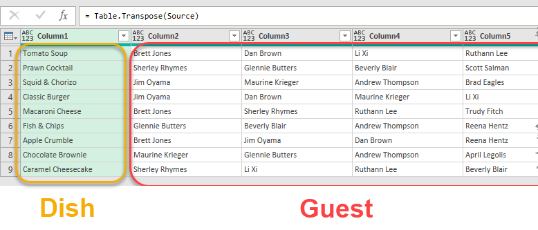
This layout is cool for Unpivot!

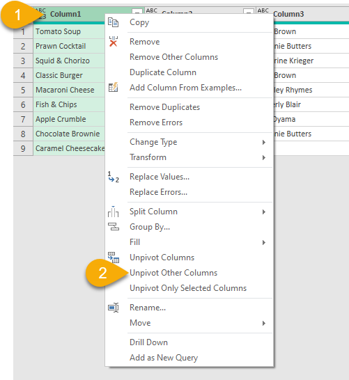
1. Right-Click Column 1 header
2. Unpivot Other Columns (note: this is important because we don’t know how many guests (columns) we will have every time, but we are pretty sure we will have only one columns of “Dish”)

And now, we have a “Tabular” layout instead.  A dish will repeat itself in Column1 for all guests who picked it.

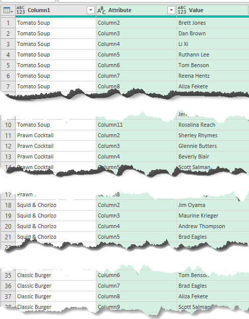
Let’s do some tidy up before we go to the next transformation.

The next step is to “LOOKUP” the type of each type.  As an Excel guy, you should know VLOOKUP… but in Power Query, it is “Merge” queries.

Merging the “Output1” query to the “Dish” query

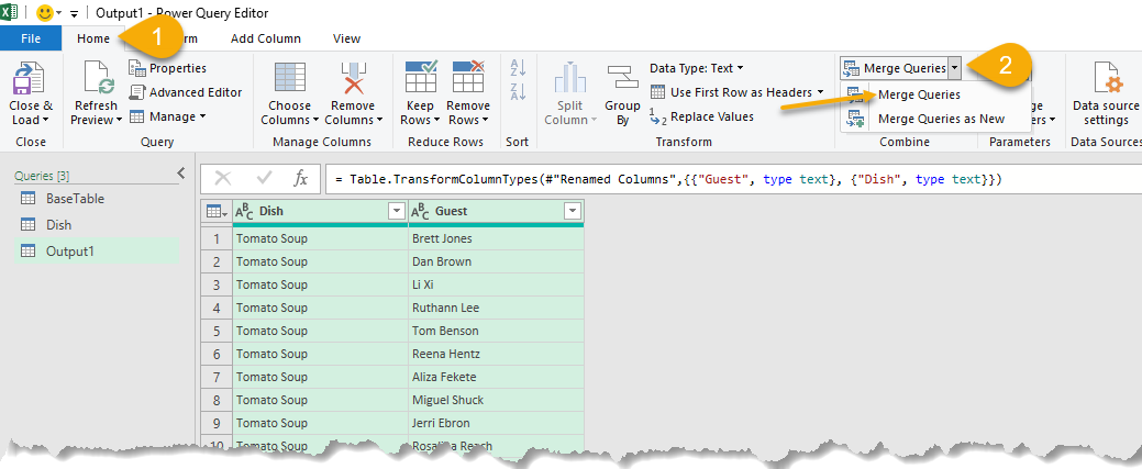
1. Go to the Home tab
2. Click the dropdown menu of “Merge Queries”, select “Merge Queries“

In the Merge queries dialog box, select as follow: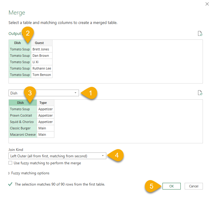

In plain English, it tells Excel to merge the Output1 table with Dish table by using the common column “Dish” in both tables. Based on a all rows from the first table (Output1), returns all matched rows from the second table (Dish).

Now, we should have the following:

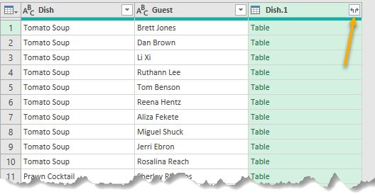
Click that “Expand” icon on the column header of “Dish.1” and select the column we want.

Let’s see it in action:

walala!  There we go!  A tabular table with Dish, Guest, and Type on three columns 🙌🏻

With this layout, Pivot it to our expected output is just a piece of cake. 🙂

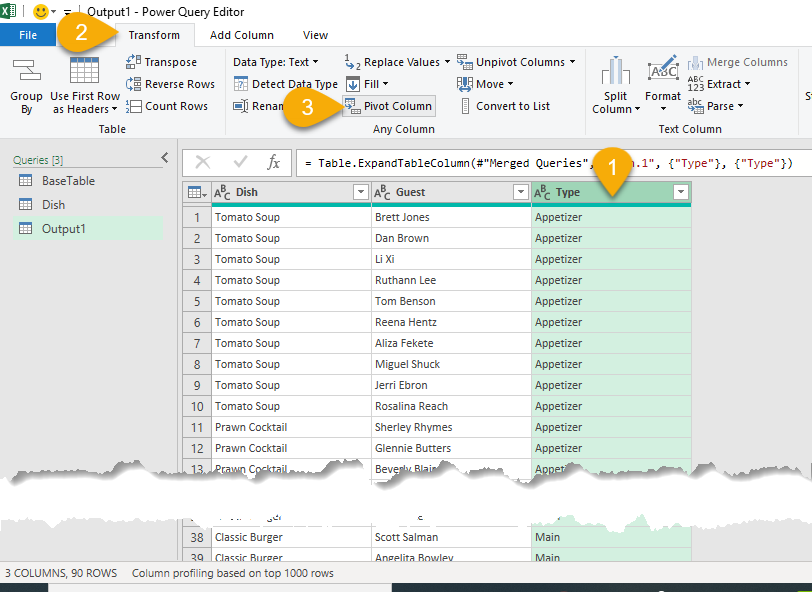
Pivot the column “Type”

1. Select the column “Type“
2. Go to Transform tab
3. Pivot Column

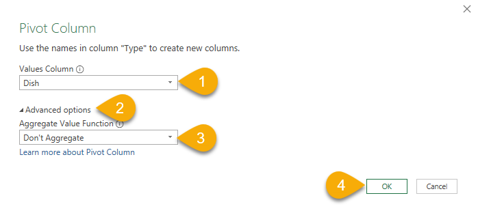
In the Pivot Column dialog box, select as follow:

1. Select “Dish” as Values Column (telling Excel to put the “Dish” under pivoted rows/columns)
2. Expand the Advanced options
3. Select “Don’t Aggregate” (telling Excel not to do any calculation; simply put the values into corresponding rows/columns)
4. OK

What a magic!?

We have the Output1 ready!  First challenge solved.

D. Counting the number of each dish

At this point, to count the number of each dish is relatively easy.  We can ride on the steps on Output1 to start.

1. Right-click Output1
2. Duplicate

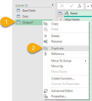
Let’s rename the duplicated query to Output2

We can ride on the steps before “Changed Type“.

1. On the Query Setting pane, right-click the step “Changed Typed”
2. Delete Until End

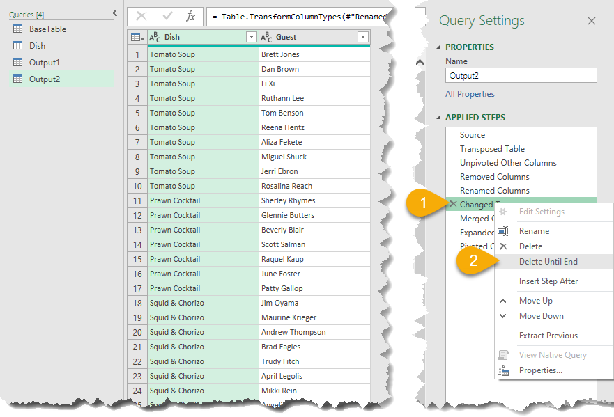
As you see, from there we have a simple table with two columns: Dish and Guest.

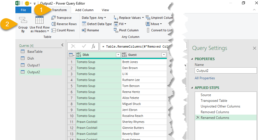
Now we can do the counting by using Group By

1. Go to Transform tab
2. Group By

In the Group By dialog box, select as follows: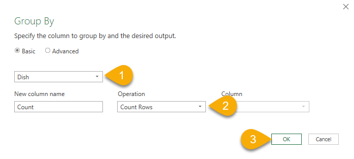

(Note: New column name is a free input for the new column name.  You may change it if you want to.)

HERE WE GO! 

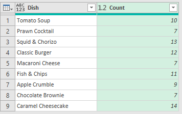
Challenge two is done!

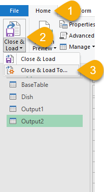
E. Load the results to worksheet

1. Go to Home tab
2. Close and Load
3. Close & Load To…

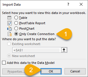
We are not loading it to Table at this point because we have four queries in total.  If we load to Table now, the four queries will be loaded on four separate worksheets as four different tables.  That’s why I select “Only Create Connection” here.

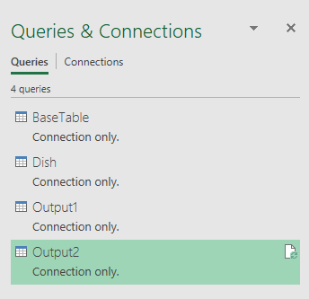
Now, on the Queries & Connections pan on the left, we should see four queries there.

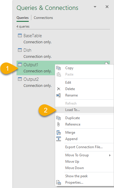
To load the Output1 / Output2 to spreadsheet,

1. Right-click Output1 / Output2
2. Load To…

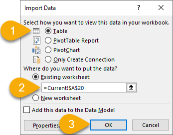
In the Import Data dialog box, select as follows:

1. Table
2. Where you want to put it on
3. OK

MISSION ACCOMPLISHED!

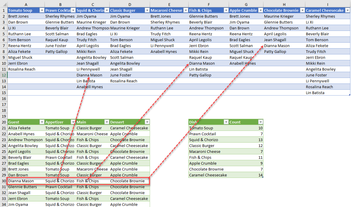
Let’s test it by adding new guest:

Simply awesome! 😎

You may download a sample workbook with all the queries HERE.

Hope you like it.

The above involves lots of steps and procedures.  I believe it’s better to demonstrate it with a video, which is under production now available.

In the video, I will also talk about how to handle if a guest pick multiple items for the same types, e.g. what if A guest picked two desserts?  The output should say… “Multiple items selected, please double check”, something like that…

Meanwhile, please leave your comments and let me know what you think about this approach.  Or if you’d like to share your solutions too.