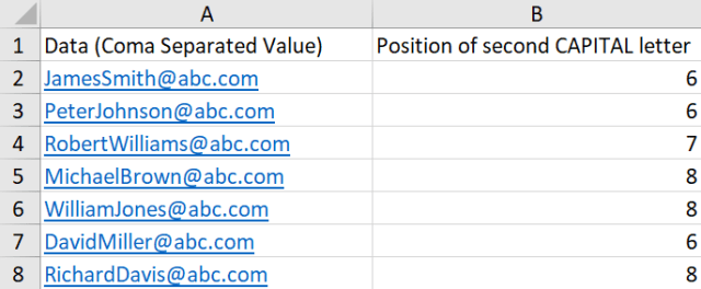
In the previous blog post, we see how Flash Fill extracts First Name and Last Name from an email address in a format shown above. I’ve also recorded a video for that post.
Flash Fill is so smart to detect the pattern of CamalCase and return the desired result in a flash. However, if you are still using Excel 2010 or before, it is NO EASY TASK and required advanced skills in formula writing. The key challenge is to identify the position of the second CAPITAL letter in the text string. Once we have identified the position of it, getting the First Name and Last Name is totally manageable.
Here’s the formula to identify the position of the second CAPITAL LETTER:
{=MATCH(TRUE,CODE(MID(A2,ROW(INDIRECT("2:"& FIND("@",A2)-1)),1))<=90,0)+1}
Note: This is an array formula, requiring Ctrl+Shift+Enter
How the formula works? I am not going to explain in super details about all functions involved, but I will walk you through the major steps.
First, get a list of sequential numbers from 2 to the position before “@”
ROW(INDIRECT("2:"& FIND("@",A2)-1)

This formula is typically used to generate an array of sequential numbers. E.g.
ROW(INDIRECT(“2:5”) will return an array of {2;3;4;5}.
By making it dynamic to the position of “@”, & FIND(“@”,A2) – 1 is used instead of a hard-coded number.
Note: I intentionally start with 2 in order to skip the first letter, which is always a capital letter in our case.
Second, extract all single letter from the list
This is achieved by feeding the prior formula into MID.
MID(A2,ROW(INDIRECT("2:"& FIND("@",A2)-1)),1)
And we will have the following as a result:
Tip: To evaluate a result in the formula bar, select the portion of formula and then press F9. Press ESC to go back to the original formula
Third, convert the letters into computer codes
This is achieved by using the function CODE.
CODE(MID(A2,ROW(INDIRECT("2:"& FIND("@",A2)-1)),1))

Forth, compare the codes with 90
CODE(MID(A2,ROW(INDIRECT("2:"& FIND("@",A2)-1)),1))<=90
A-Z are stored as from 65 to 90, while a-z are stored as from 97 to 122, in most of the computer, if not all. That’s why if it is <=90, it is a CAPITAL LETTER.
Note: Try input =CODE(“A”) in a blank cell to see the result
As a result, Excel gives an array of TRUE/FALSE where TRUE indicates a CAPITAL LETTER.

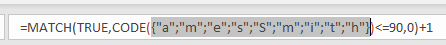
Fifth, locate the position of TRUE using MATCH
MATCH(TRUE,CODE(MID(A2,ROW(INDIRECT("2:"& FIND("@",A2)-1)),1))<=90,0)
This is quite straight forward, and it returns t the following result:

Sixth, offset the result by +1
Remember we intentionally omitted the first letter? That’s why we need to add one to offset it.
=MATCH(TRUE,CODE(MID(A2,ROW(INDIRECT("2:"& FIND("@",A2)-1)),1))<=90,0)+1

As a result, we’ve got the position of the second capital letter. Make sense?
IMPORTANT: As this is an array formula, we have to input the formula with CTRL+SHIFT+ENTER
Once we’ve got the position of the second capital letter, the rest would be easy.
You may download a Sample File to follow along.
In the sample file, there is also a solution for Excel 365 users with dynamic arrays.
Hope you like it. 🙂
Want to read more about other applications of the functions discussed? Check it out:
LEFT: https://wmfexcel.com/tag/left/
MID: https://wmfexcel.com/tag/mid/


