Convert text of specific pattern like “1d 2h 3m 4s” into real time (26:03:04) in Excel

To kick start the Year of Monkey, let’s challenge the apparently impossible…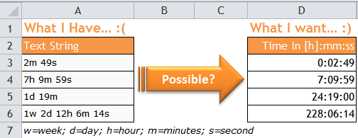

Do you think it is not possible in Excel?  If you do, you are absolutely normal. 🙂

In fact, the solution for this may be much shorter than you may have expected:

=SUMPRODUCT(IFERROR(MID(" "&A3,SEARCH({"w","d","h","m","s"}," "&A3)-2,2),0)*{604800,86400,3600,60,1})*(1/24/60/60)
'where A3 is the cell holding the text string

To understand how it works, bear in mind one simple goal:

To find out how many “seconds” represented in the text string.

Once we know how many seconds it is talking about, converting it into an Excel recognizable time is just a piece of cake (or easier than eating lettuce, in Cantonese).

Before we start:

Excel 101 – What is time?

“TIME is a value ranging from 0 (zero) to 0.99988426, representing the times from 0:00:00 (12:00:00 AM) to 23:59:59 (11:59:59 P.M.). ”  from Excel Help.

Every second is divided evenly.  Hence in Excel,  the value for 1 second is 0.0000115740740740741, which is basically 1/24/60/60.  (24 hours a day, 60 minutes an hour, 60 seconds a minute)

By understanding the basics, we may dive into the formula and see how it works.

Let’s focus the text string in A5 and A6 for illustration:

Step 1 – Get the corresponding numbers for “w”, “d”, “h”, “m”, “s”

MID(" "&A6,SEARCH({"w","d","h","m","s"}," "&A6)-2,2)

This formula search for each character in the text string and then extract the two letters before the character.  

Note: A prefix ” ” (space)  is added to the original text.  This trick ensures no error is returned for the first set of information carrying one digit only.

The resulting array as follow:

{" 1"," 2","12"," 6","14"}

When there is absence of a particular character, e.g. no “w”, “h” and “s” in A5 where the text string is “1d 19m”, the resulting array is returned:

{#VALUE!," 1",#VALUE!,"19",#VALUE!}

To handle such possible error, it is wrapped by IFERROR(value,0):

IFERROR(MID(" "&A5,SEARCH({"w","d","h","m","s"}," "&A5)-2,2),0)

As a result, the formula returns the following arrays:

{0," 1",0,"19",0} for text string "1d 19m"
{" 1"," 2","12"," 6","14"} for text sting "1w 2d 12h 6m 14s"

Step 2 – Calculate how many seconds

To multiply the resulting elements in the above array by the corresponding numbers of seconds, i.e. 

*{604800,86400,3600,60,1}
where 604800 seconds in a week; 86400 seconds in a day,
3600 seconds in an hour, 60 seconds in a minutes, 
and of course 1 second in a second.  
We need to put 1 as we need this array to be of the same size as the one returned.

To add the product of the arrays without using Ctrl+Shift+Enter, I use SUMPRODUCT  (what else?)

SUMPRODUCT({0," 1",0,"19",0}*{604800,86400,3600,60,1}) 
==> 0*604800 + " 1"*86400 + 0*3600 + "19"*60 + 0*1
= 87540
'for "1d 19m"

SUMPRODUCT({" 1"," 2","12"," 6","14"}*{604800,86400,3600,60,1}) 
==> " 1"*604800 + " 2"*86400 + "12"*3600 + " 6"*60 + " 14"*1
= 821174
'for "1w 2d 12h 6m 14s"

Are they returning the number of seconds described by the text string? oh YES!

Step 3 – Convert the number to a value that Excel understands as second

Simply multiplying the number by the representing value of a second in Excel.

87540*(1/24/60/60) =  1.013194444 ==> 24:19:00 'for "1d 19m"
821174*(1/24/60/60) =  9.504328704  ==> 228:06:14 'for "1w 2d 12h 6m 14s"

IMPORTANT:

Format the cells as [h]:mm:ss

The formula works when the following the assumptions are true:

• The numbers are up to 2 digits
• There should be at least one space between each subset
• No space with subset

Example: “1 w2d 12 h6m 14 s” is not going work… 😦

Note: The sequence of “w”, “d”, “h”, “m”, “s” does not matter in the calculation but it is always a good practice to keep logical flow.

Final Note:

I have been talking about this again and again in various posts.  Why complicating thing at the begining?  Whenever possible, keep input simple and organized.  One simple rule: One Cell One thing.

Want more TIME?

• Do you need TIME?
• Time Conversion – How to convert 24hr input as 4-digit number into TIME in Excel?
• Time Conversion (2)
• SUM Time in the end of text strings
• How to limit time interval input in a single cell?