Got the following question from a reader:

Under data validation, is it possible for me to restrict the time duration (in a cell) to be 30mins or less?

Example:
9.00 – 9.30 (accepted)
10.15 – 10.50 (rejected)

Obviously, the answer is YES.

Assume the input cell starts from A1,

Select A1

• Go to Data –> Data Validation
• On Settings, Allow Custom
• 
• Input the following formula:

=MOD(TIME(MID(A1,FIND(".",A1,5)-2,2),MID(A1,FIND(".",A1,5)+1,2),)-TIME(LEFT(A1,2),MID(A1,FIND(".",A1)+1,2),),1)<TIME(,31,)TIME(,30,59)
'Thanks Haz for a more robust solution in the comment!

• OK
• Copy A1 down according to your requirement

Limitation:

The input must be in the format of h.mm – h.mm, note the space before and after the hyphen

The formula looks complicated but it is essentially

=MOD((End Time - Start Time),1)<TIME(,30,59)

MOD((End Time – Start Time),1) is used to calculate the time difference that allows End Time falling onto next day.  To learn more about this trick, please refer to the blogpost by Gašper Kamenšek.

The result is then compared to TIME(,31,) TIME(,30,59), i.e. the numeric value of 31 minutes 30 minutes 59 seconds.  When it is less than 31 minutes 30 minutes 59 seconds, it is “good enough” should cater all the minutes around the clock to say the period input is 30 minutes or less (provided that second is not an consideration).   Thanks again to Haz for the suggestion! 🙂

The expression <=TIME(,30,) should be more intuitive.

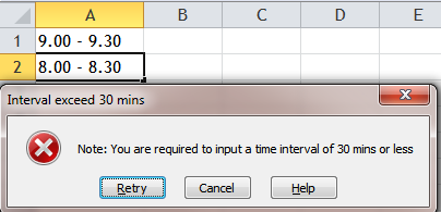
However I do not have a solution to avoid the rounding issue for such cases as 08.00 – 8.30 which “incorrectly” reject your input when you set the comparison to <=TIME(,30,).

Please leave your comment if you have a solution for this.

Side topic for discussion:

Many users used to input a range of whatever values (be it time, date, or just simple number) into a single cell, using a hyphen in-between.   For example:

• 8:00-9:00
• 20/12/2015-25/12/2015
• 100-200

Maybe it is easier to input (which I really doubt).  This is absolutely NOT what is expected to use Excel as a analytical tool.  Why? Because the cost of it is much higher than the benefit you enjoy.

Take a look at the solution above.  The monster formula is a result of this bad practice.

If the Start time and End time (in correct time format) are input into two different cells, say A1 and B1 respectively.  The solution could be as simple as

=MOD((B1 - A1),1)<TIME(,31,)TIME(,30,59)

Although it is very likely that you may write a “super (long)” formula to fix your problem, why create a problem you can avoid easily at the first place?

Whenever possible, stick to a simple rule: One cell, One thing.