This should be the last post in 2015. So it’s better to answer unanswered question in the year. 🙂
Question: “VLOOKUP will return the first matched value found, in case there are multiple matched records what formula should we use?”
This can be achieved by using VLOOKUP with a helper column, or by complicated array formula. VLOOKUP with helper column is my preference not only because it is easier to construct, but also (and mainly) because most users with experience in writing formula would understand it. I think the latter is important. It is better using a formula that you (and other regular users) can modify according to your need than seeking help from time to time.
Let’s take a look at the demonstration below:
You may download a Sample File to follow along.
The formula in G2:
=VLOOKUP(F2&"|"&E2,$A$2:$C$13,3,FALSE)
Yes. It is as simple as that. You may notice that the table_array starts in column A instead of column B. That hidden column is essential and it makes the VLOOKUP of multiple matched record easy.
Let’s examine what is hidden: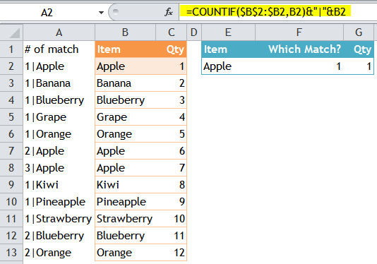
In A2,
=COUNTIF($B$2:$B2,B2)&"|"&B2 'copy down
This formula creates a unique value for VLOOKUP.
- The COUNTIF($B$2:$B2,B2) tells us the number of occurrence of an item on the list. (Note the absolute reference $B$2 and the relative row reference $B2 in the range for COUNTIF);
- The &”|”&B2 then gives you the unique value for VLOOKUP.
With the helper column, VLOOKUP the Nth matched record is a piece of cake.
=VLOOKUP(F2&"|"&E2,$A$2:$C$13,3,FALSE)
- F2&”|”&E2 is the lookup_value i.e. which item and which one (the same structure used in the helper column)
- $A$2:$C$13 is the table_array (it starts from column A, not B)
- The column_index is 3 (not 2 because it starts from column A)
- FALSE (or 0) in the final argument for exact match.
Tip: To stay in the same cell after Enter, press Ctrl+Enter
Final notes:
- #N/A means the item you input and the case of match does not exist on the table. You may replace the #N/A with any messages by using IFERROR;
- If you apply this technique to a really large table, speed may suffer.
Now it’s time to turn off your computer. It’s Christmas Eve.
Sincere wishes to all of you and your beloved ones!
Merry Christmas
&
Happy New Year!
See you in 2016 🙂


