Situation:

In a filtered range of data, we made few changes on the side. Then we want to replace the original values with the updated values.

What action appear on top of your mind? Copy and Paste of course.

But… if you had tried, you knew it… a regular Copy and Paste does NOT work. 😓

Did you see the problem?

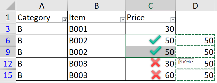
At the first glance, It looks like that only 2 values were replaced correctly. Indeed the result was a total mess (only the first cell will be pasted with the value as expected).

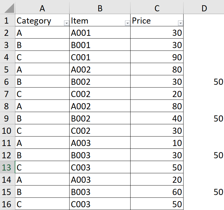
Let’s clear the filter and examine what’s actually been pasted (assuming we spotted something wrong and checked immediately… you know what I am talking about).

😨😨😨 OMG… What happened?

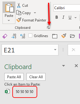
When we copy from a filtered range, only “Visible cells” are copied. It is denoted by the “marching ants” as shown below:

In this case, four values (cells) are copied to clipboard. Excel simply ignores all the cells (values) that are filtered out.

When we paste this to C6, Excel pastes these four values as a continuous range starting at C6. In other words, the four values will be pasted to C6, C7, C8 and C9 respectively. That’s why the copy and paste in filtered range is a hassle.

We have a problem. Do we have a solution?

Not really a solution, but workaround for situation like this.

The secret sauce is “Skip Blank”.

Let’s follow the steps below:

You download a sample file to follow along.

1. Clear all filters before copying

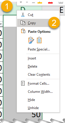
2. Copy the whole column (D)

3. Paste Special… to the destination column (C)

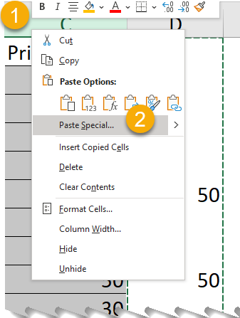
4. Paste “Values” and most importantly check “Skip blanks”

OK! 🌭🌭

Let’s watch it in action. (Note: targeted cells are highlighted for easy reference)

As simple as this. 😉

Watch it in action here:

Related blogposts:

Hidden Rows vs. Filtered Rows

Using Skip blanks in Paste Special