I really like Power Query (in both Excel and Power BI).  Honestly I do not know much about the M behind the scene (still learning it piece by piece).  Nevertheless, I’ve got the POWER simply through the User Interface of Power Query Editor.  Seriously,  everyone can become a data wizard by using Power Query!  Let’s watch the following two videos to feel the POWER of Power Query.

Here’s is a challenge (with solution) from Mr Excel on how to reshape data.

You may download a sample workbook from Mr.Excel YouTube channel to follow along.

And here’s my approach to solve the challenge:

If you prefer reading to watching, please continue to read this post.

Note: All screenshots used in this post are captured using Excel for Office 365.  If you are using other versions of Excel, you may find the locations and look&feel of buttons a bit different. The concept is the same though.

Here’s the challenge – Reshaping the data

A picture tells thousand words:

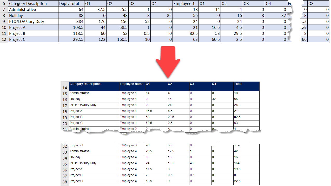
Before Power Query, the first thing in my mind is…

OMG…. seriously? Do i have to re-shape the data by manual Cut and Paste?  How many columns do we have?  Is it one-off task? Reoccurred tasks with new data?

With Power Query, these questions bother me no more! 🙂

Here’s the step-by-step solution:

A. Turn the table into Excel Table

1. Select the range of data (A5:Z11) in our example
2. Go to Insert tab
3. Select Table
4. Uncheck “My table has headers”
5. Click OK

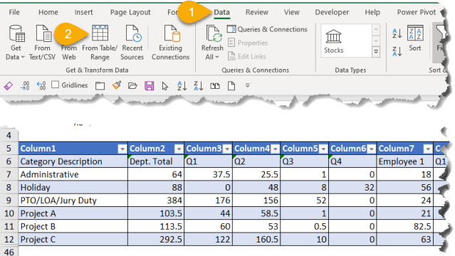
B. Load the Excel Table to Power Query

Select any cell of the Table just created…

1. Go to Data tab
2. Select From Table/Range

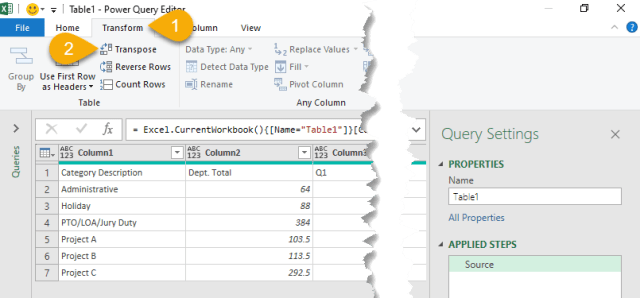
C. Transpose the Table

This is our first transformation.

1. Go to Transform tab
2. Select Transpose

Now it’s the time to make a promotion 🙂 To promote the first row as header:

1. Go to Home tab
2. Select Use First Row as Headers

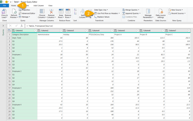
Now we’ve got a much better layout 🙂

If you are experienced in preparing data for pivot table, you should know that grand totals and/or subtotals are not necessary in the dataset.  Same case here!  We will remove those grand totals and subtotals later.

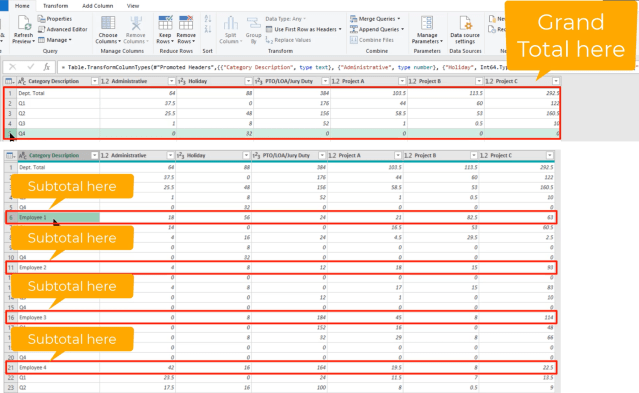
D. Remove Grand Totals

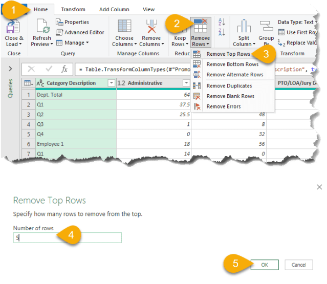
To remove the grand totals in this case is easy.  Simply remove the top 5 rows:

1. Go to Home tab
2. Select Remove Rows
3. Select Remove Top Rows
4. Input 5 
5. OK

Nevertheless we need further steps before we can remove the subtotals.

E. Split the Employee from Quarter; and Add a column for Employee

As a general rule, we should have more than one information under one column.  In our dataset we now have both Employee and Quarter under the same column “Category Description” (we will rename this header later).  This is no good.  We need to separate Employee from this column and create an column of Employee alone.

Let’s do it:

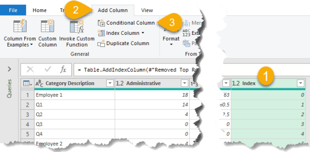
1. Go to Add Column tab
2. Click Index Column

A new column called “Index” is added.  You will see a list of sequential number from 0 to 19 there.  Nevertheless, this sequential list doesn’t help much at this stage.  Look at the dateset, our records are organized in a way of 5 rows per record, with the first row being the employee name and the subtotal.  So a list of repeating pattern from 0 to 4 would help!

Let’s further transform the Index column to get what we need:

1. Select the Index column
2. Go to Transform tab
3. Select Standard
4. Select Modulo
5. Input 5
6. OK

What Modulo does?

Based on the value input, the function Module will give the remainder for each value in the column.  For a sequential list from 0 to 19, this function returns a list of 0 to 4 repeatedly.

Think about this:

• 5 divided by 5 –> Remainder is 0
• 6 divided by 5 –> Remainder is 1
• 7 divided by 5 –> Reainder is 2
• …
• 10 divided by 5 –> Remainder is 0
• 11 divided by 5 –> Remainder is 1
• …

Make sense?  As a result, the Index column become this:

Now we need another helper column to extract the employee name:

1. Select the Index column
2. Go to Add Column
3. Select Conditional Column

Then input the Condition and Output as below:

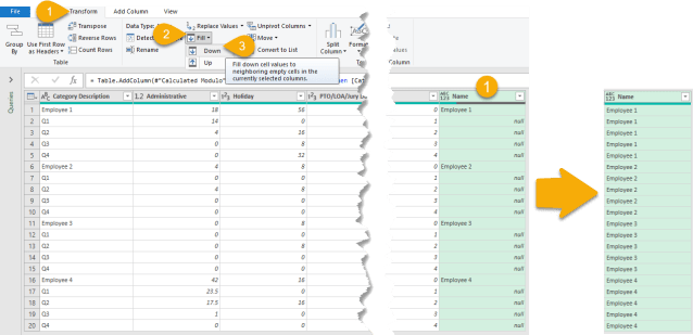
With the new column “Name” just created, we’ve got the employee name correctly on each row with “0” in the Index column.  We need to fill the gap:

1. Select the Name column; Go to Transform tab
2. Select Fill
3. Select Down

F. Remove Subtotals

With the two helper columns added in the previous section, we are now ready to remove the subtotals:

1. Click the pull down icon on the header of “Index“
2. Uncheck 0
3. OK

Let’s rename the columns by double-clicking the header:

The column Index is no longer require.   Right-click on the header and Remove it.

Thanks for its contribution! 👏

G. Unpivot Columns other than Employee and Quarter

1. Select the column Quarter
2. Also select the column Name (by holding Ctrl key)
3. With the two columns selected, right-click on the header –> Unpivot Other Columns

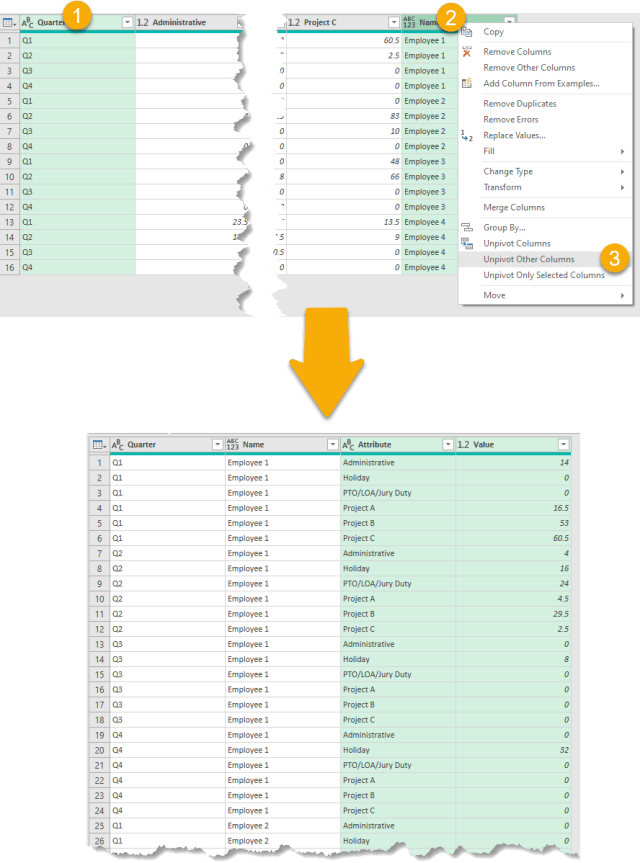
Rename “Attribute” to “Category”

Tip: Now we’ve got a layout that is ideal for various data analysis and pivot table.  We may stop here and get the required output by using Pivot Table.  Please read the bonus part of my video for more details.

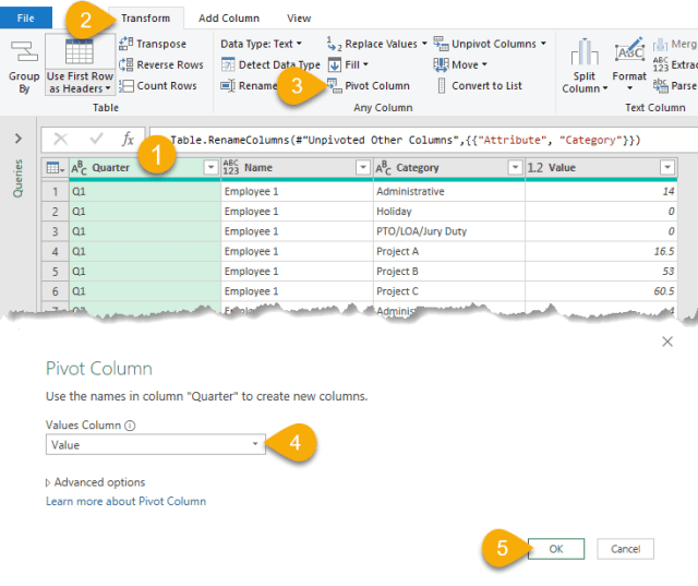
H. Pivot Column

1. Select the column Quarter
2. Go to Transform tab
3. Select Pivot Column
4. In the Pivot Column dialog box, Select Value
5. OK

Almost there…

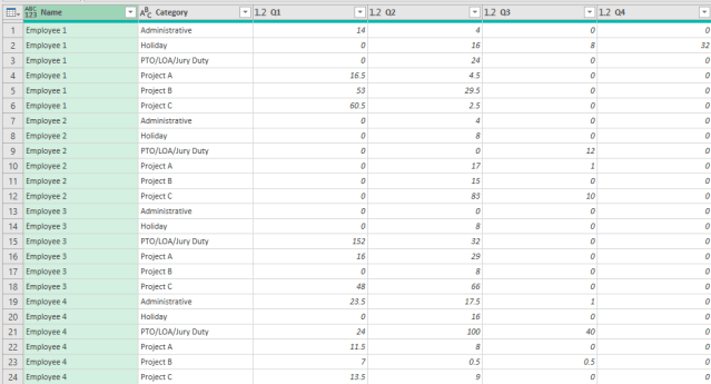
We need the total column for four quarters.

Let’s do it:

1. Select the four columns Q1 to Q4 (tip: hold SHIFT key for selecting adjacent columns)
2. Go to Add Column tab
3. Select Standard
4. Select Add (so obvious 😁)

Remember to rename to added column from “Addition” to “Total”

To make the final output 100% matched with the requirement, let’s re-order the columns by drag and drop:

Final touch-up, define the date type.

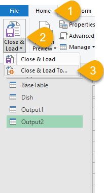
I. Close and Load

Now we are ready to load the output to spreadsheet!

1. Go to Home tab
2. Select Close and Load
3. Select Close and Load to…

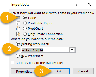
In the subsequent dialog box:

1. Select Table
2. Select Existing worksheets: and input the cell reference where you want to load the result
3. OK

Here we go! Enjoy!

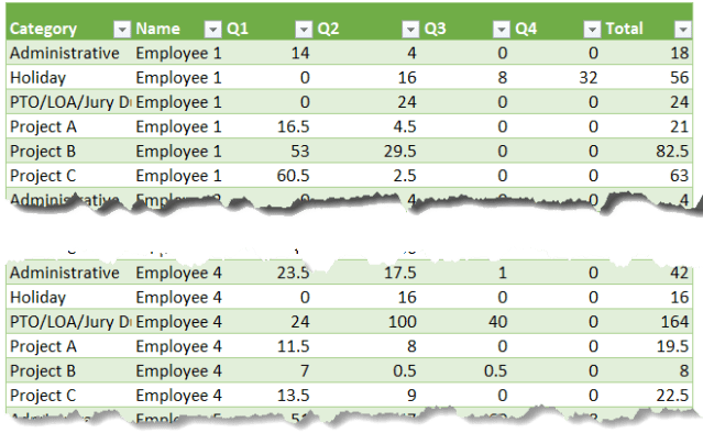
As you see, we can do the data-reshaping all the way with Power Query’s UI only.  Not a single line of code written.  Isn’t it cool? 😎

Although we can finish the transformation with Power Query, I’d highly recommend we stop at section G because the resulting layout there is ideal for further analysis.  We can do it with regular Pivot Table with more flexibility to end users, provided that end users know how to use Pivot Table. 😉

You may watch the bonus session in the video to learn more.

I hope you can feel the POWER of Power Query and start falling in love with it.

Click HERE to download the sample file with the solution.