Making cell border in #Excel should be something really basic. However, some people may have found it frustrating/confusing to play Hide and Seek with borders just hoping that they will be displayed in the way they want it.
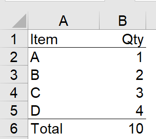
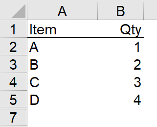
For example, a simple table as below, we have Bottom Border on row 5 (or A5:B5 in our example):
When we hide row 5, the border line is gone….
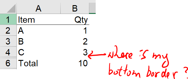
It is hidden indeed. Did we just hide row 5? 🙂
If you don’t know Excel well, you may reapply the Bottom Border on row 4 again to get back the visual effect that you’d like to have.
However, if you do this, you will see “extra” border when you unhide the row 5 later. Probably it is not something that you want.
In this example, as we want to show the border between items and Total, we should apply Top Border to cell A6:B6 instead.
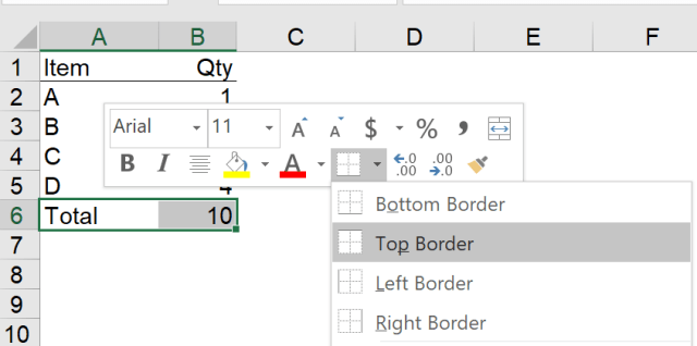
When Top Border is applied to A6:B6, we’ll see the border as long as the row 6 is there.
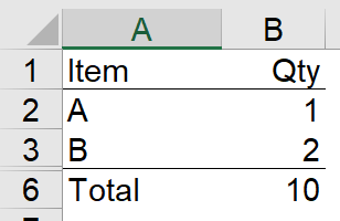
But, you should be aware of this by now… if row 6 is hidden, the border is not displayed either.
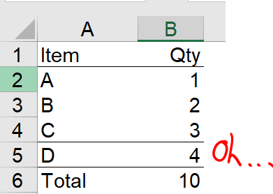
This could be something that you want… But just in case it is not, that means you want to see the Bottom Border at the end of the items. You may think it’s quite troublesome for a user to determine whether s/she should apply Bottom Border to A5:B5, or Top Border to A6:B6, or indeed both in this case.
Actually we could select two rows of cell (i.e. A5:B6 in our example), then apply “middle” Border.
By doing so, we have applied Bottom Border to A5:B5 and Top Border to A6:B6 respectively, at the same time.
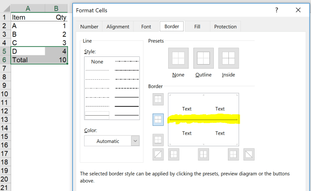
The only way to identify whether a border belongs to a cell is to see it from “Format Cells” dialog box. Right click on a cell, select Format Cells… go the the “Border” tab. There you go.
Remember, when you hide a cell, you hide border(s) that belongs to it.
p.s. No sample file accomplished for this post. Suggest you experiment it from a blank Excel sheet. 🙂


